Basic Signal Manipulation and Representation

1.3 Basic Signal Manipulation and Representation

This section discusses basic tools for mathematically representing and manipulating signals. The motivation is that it is important not only being knowledgeable on manipulating signals using software, but also algebraically, developing expressions and theoretical analysis.

1.3.1 Manipulating the independent variable

Many signal processing tasks require manipulating $t$ (for continuous-time signals) or $n$ (for discrete-time). A convenient way to introduce this manipulation is by using examples. Define the signal $x [n] = n^{2}$ for $n = 3, 4, 5$ and 6, and zero otherwise. This signal has only four non-zero amplitude values: $9, 16, 25$ and 36,’ at $n = 3, 4, 5$ and 6, respectively. The task here is to find new signals based on $x [n]$ , namely: $y_{1} [n] = x [n - 2]$ , $y_{2} [n] = x [- n + 3]$ , $y_{3} [n] = x [2 n]$ and $y_{4} [n] = x [n^{2}]$ .

An interpretation of $y_{1} [n] = x [n - 2]$ is that it is a sequence of events that is related to the original (“mother”) sequence $x [n]$ but with a time difference. For example, if $n = 6$ is interpreted as 6 o’clock and $x [6] = 36$ is the heart rate of an animal at that moment, the same measurement $y_{1} [8] = 36$ is found at $y_{1} [n]$ but two time units later (8 o’clock). Hence, the notation $y_{1} [n] = x [n - 2]$ indicates that $x [n]$ and $y_{1} [n]$ present the same ordinate (in this case, amplitude) values, but these values occur two samples later in $y_{1} [n]$ when compared to $x [n]$ .

One can create a mapping such as Table 1.2, which fills up the first column with values of $n$ in the region of interest. Then, it is simple to get columns for $n - 2$ , $- n + 3$ , $2 n$ and $n^{2}$ . Columns $y_{1} [n], y_{2} [n], y_{3} [n]$ and $y_{4} [n]$ are filled up based on the auxiliary columns $n - 2$ , $- n + 3$ , $2 n$ and $n^{2}$ , but they correspond to amplitudes at the value of $n$ given in column 1. For example, the second row indicates that $y_{1} [- 2] = 0, y_{2} [- 2] = 25, y_{3} [- 2] = 0$ and $y_{4} [- 2] = 16$ .

Table 1.2: New signals

y_{1} [n] = x [n - 2]

y_{2} [n] = x [- n + 3]

y_{3} [n] = x [2 n]

and

y_{4} [n] = x [n^{2}]

, obtained by manipulating

x [n] = n^{2} (u [n - 3] - u [n - 7])

$n$	$x [n]$	$n - 2$	$y_{1} [n]$	$- n + 3$	$y_{2} [n]$	$2 n$	$y_{3} [n]$	$n^{2}$	$y_{4} [n]$
$- 3$	$0$	$- 5$	$0$	$6$	$36$	$- 6$	$0$	$9$	$0$
$- 2$	$0$	$- 4$	$0$	$5$	$25$	$- 4$	$0$	$4$	$16$
$- 1$	$0$	$- 3$	$0$	$4$	$16$	$- 2$	$0$	$1$	$0$
$0$	$0$	$- 2$	$0$	$3$	$9$	$0$	$0$	$0$	$0$
$1$	$0$	$- 1$	$0$	$2$	$0$	$2$	$0$	$1$	$0$
$2$	$0$	$0$	$0$	$1$	$0$	$4$	$16$	$4$	$16$
$3$	$9$	$1$	$0$	$0$	$0$	$6$	$36$	$9$	$0$
$4$	$16$	$2$	$0$	$- 1$	$0$	$8$	$0$	$16$	$0$
$5$	$25$	$3$	$9$	$- 2$	$0$	$10$	$0$	$25$	$0$
$6$	$36$	$4$	$16$	$- 3$	$0$	$12$	$0$	$36$	$0$
$7$	$0$	$5$	$25$	$- 4$	$0$	$14$	$0$	$49$	$0$
$8$	$0$	$6$	$36$	$- 5$	$0$	$16$	$0$	$64$	$0$
$9$	$0$	$7$	$0$	$- 6$	$0$	$18$	$0$	$81$	$0$

Example 1.2. Time-reversal of signals. The operation $y [n] = x [- n]$ corresponds to flipping the signal over the ordinate axis. In Matlab/Octave it can be implemented with fliplr (left-right) or flipud (up-down) for row and column vectors, respectively. For example, assume that $x [n]$ has amplitudes $3, 4$ and 5, at time instants $n = 0, 2$ and 4, respectively (after discussing the impulse $δ [n]$ in Section 1.3.4, we will describe this signal as $x [n] = 3 δ [n] + 4 δ [n - 2] + 5 δ [n - 4]$ ). One can represent $x [n]$ as the row vector x=[3 0 4 0 5] and flip it using y=fliplr(x) in Matlab/Octave. It is important to note that, when representing a signal, one vector can store the amplitude values but not their respective time instants. An additional vector is required to store the time information. Listing 1.2 is a snippet (part of the script) used to generate Figure 1.5. It illustrates the care that must be exercised to properly represent the signals $y [n] = x [- n]$ using a computer program. Note that the user must relate the amplitude vector and the “time” vector.

Listing 1.2: MatlabOctaveCodeSnippets/snip_signals_timereversal.m. [ Python version]

1x=[3 0 4 0 5]; %some signal samples 
2y=fliplr(x); %time-reversal 
3n1=0:4; %the 'time' axis 
4n2=-4:0; %the 'time-reversed' axis 
5subplot(211); stem(n1,x); title('x[n]'); 
6subplot(212); stem(n2,y); title('y[n]');

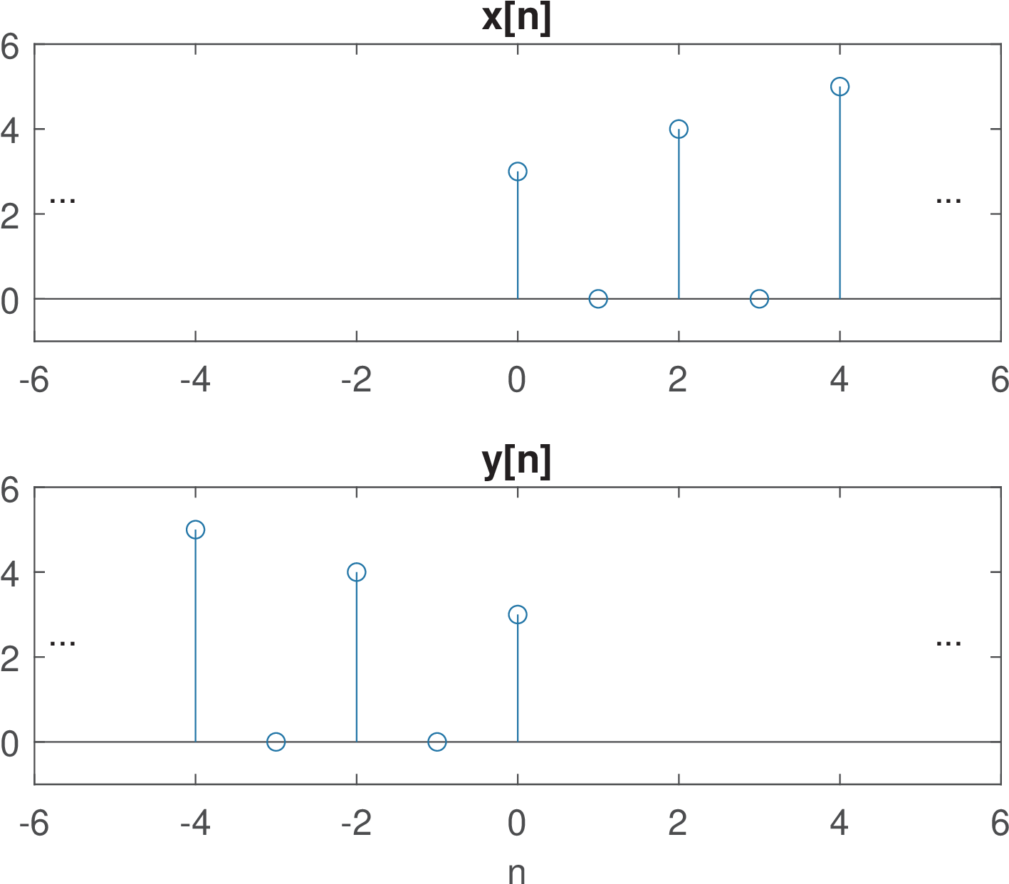
Figure 1.5 was produced using three dots to indicate that the signals have infinite duration in spite of being represented by finite-length vectors. Another convention is that, when an amplitude value is not explicitly shown, it is assumed to be zero. $□$

1.3.2 When the independent variable is not an integer

Almost all manipulations of $t$ are equally applied to manipulating $n$ of discrete-time signals. But a discrete-time signal $x [n]$ is undefined if $n \notin ℤ$ (e. g. $x [1.5]$ in undefined).

For instance, $x [2 n]$ behaves slightly different than $x (2 t)$ given that the discrete-time signal is not defined for non-integer $n = \pm 0.5, \pm 1.5, \pm 2.5, \dots$ . Therefore, only the amplitude values of $x [n]$ for $n$ even are present in $x [2 n]$ , while the values for $n$ odd are discarded.

Using a similar reasoning, when dealing with a discrete-time signal $y [n] = x [n ∕ 2]$ , it is important to adopt a definition such as:

y [n] = {\begin{matrix} x [n ∕ 2], & when n ∕ 2 is an integer \\ 0, & otherwise \end{matrix}

(1.2)

that emphasizes the assumption $n \in ℤ$ .

1.3.3 Frequently used manipulations of the independent variable

In signal processing, one is often manipulating the dependent variable (for example, multiplying the signal amplitude by two) and also the independent variable, which is the time abscissa in most cases in this text. These two ways of manipulating a variable are rather different. This section discusses manipulating the independent variable.

One can always use a procedure such as the one illustrated in Table 1.2 to obtain the signal after a manipulation of the independent variable. However, it is worth to memorize the resulting signals in two common situations. The first one is the time shift and the second situation is when simultaneously scaling and shifting the original signal. They are discussed in the next paragraphs.

Example 1.3. Time advance and delay rules of thumb.

It may be convenient to memorize the time advance and delay rules. Assuming $t_{0} > 0$ , these rules are ( $t$ and $t_{0}$ are assumed, but the same applies to discrete-time $n$ and $n_{0}$ ):

$x (t - t_{0})$ is a delayed version (right-shifted) of $x (t)$ and $x (t + t_{0})$ is an anticipated version (left-shifted) of $x (t)$ ;
$x (- t + t_{0})$ is obtained by first considering $x (t + t_{0})$ , which is obtained by advancing the signal by $t_{0}$ , and then flipping the result $x (t + t_{0})$ with respect to the $y$ -axis to obtain $x (- t + t_{0})$
$x (- t - t_{0})$ is also obtained by delaying $x (t)$ to create $x (t - t_{0})$ and then flipping this intermediate result over the $y$ -axis.

For example, $x (- t + 3)$ corresponds to finding the temporary result $x (t + 3)$ by advancing 3 units of time and then flipping $x (t + 3)$ over the $y$ -axis. Alternatively, one can think of obtaining $x (- t + 3)$ by first flipping $x (t)$ with respect to the $y$ -axis and then delaying $x (- t)$ by 3 (instead of anticipating it). However, a common mistake is to think that $x (- t + 3) = x (- (t - 3))$ , and start by delaying $x (t)$ by 3 and then flipping over the vertical axis. In case of any confusion, the safest option is to map some values of the abscissa such as Table 1.2. $□$

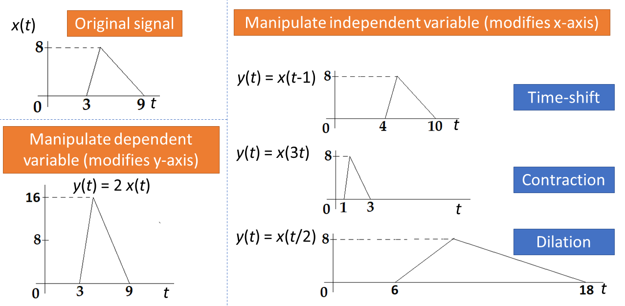
Figure 1.6 provides the example $y (t) = x (t - 1)$ of time-shift, corresponding to a delay of 1. This figure also contrasts manipulating the independent and dependent variables. In the latter case, it is the ordinate ( $y$ -axis) that is modified, with $y (t) = 2 x (t)$ changing the $y$ -axis peak value from 8 to 16. Besides, Figure 1.6 illustrates other two manipulations: contraction and dilation. Note that all three examples of manipulating the independent variable did not modify the ordinate peak value (it is equal to 8). Contraction and dilation are the topic of the next example.

Figure 1.6: Examples of manipulating the independent variable: time-shift, contraction and dilation.

Example 1.4. Time scaling rules of thumb: contraction and dilation.

Assuming that $α > 1$ , $x (αt)$ corresponds to contracting the time axis by a factor of $α$ while $x (t ∕ α)$ corresponds to a dilation by $α$ .

For instance, a pulse $x (t)$ with support⁵ from $- T_{1} ∕ 2$ to $T_{1} ∕ 2$ s leads to a total support duration of $T_{1}$ seconds, while $x (2 t)$ and $x (t ∕ 5)$ have support durations of $T_{1} ∕ 2$ s and $5 T_{1}$ s, respectively. In Figure 1.6, the original signal $x (t)$ has a support from $t = 3$ to 9 s, with a total support duration of 6 s, while $x (3 t)$ and $x (t ∕ 2)$ have supports with total duration of 2 and 12 s, respectively. $□$

Another important manipulation of the independent variable is the simultaneous combination of time-shift and scaling, discussed next.

Example 1.5. Simultaneous scale and shift rules of thumb. The signal $x (αt + β)$ , with $α, β \in ℝ$ , is commonly found in signal processing operations. It can also be found as $x ((t + γ) ∕ ξ)$ , where $γ, ξ \in ℝ$ . These two representations are related by $α = 1 ∕ ξ$ and $β = γ ∕ ξ$ . The rules of thumb are:

for $y (t) = x (\frac{t + γ}{ξ})$ , first expand or contract $x (t)$ by a factor of $ξ$ and then shift the intermediate result by $γ$ ;
for $y (t) = x (αt + β)$ , first expand or contract the original signal $x (t)$ according to the value of $α$ , then shift this intermediate result by $β ∕ α$ .

Figure 1.7 provides two examples of simultaneously scaling and shifting a signal $x (t)$ . $□$

The first example in Figure 1.7 aims at interpreting $y_{1} (t) = x (\frac{t - 3}{2})$ . One can always carefully map the signals as done in Table 1.2. But using the rule of thumb is faster. In this case, $x (t)$ can be expanded by a factor of $ξ = 2$ and the result shifted to the right (delayed) by $γ = - 3$ . Note that the support of $x (t)$ is 6, in the range $t \in [4, 10]$ . The support of $y_{1} (t)$ is $t \in [11, 23]$ , twice the support of $x (t)$ . As expected, the amplitude does not change: for both signals, it has a maximum value of 5.

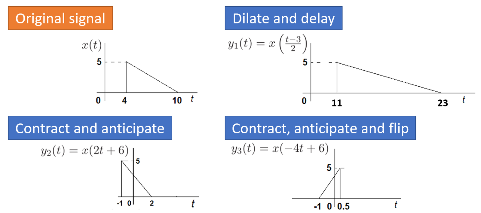
Figure 1.7: Three examples of simultaneously scaling and shifting a signal $x (t)$ .

The second task suggested in Figure 1.7 is to obtain $y_{2} (t) = x (2 t + 6)$ . One possibility is to convert the representation $x (αt + β)$ into $x ((t + γ) ∕ ξ)$ and proceed as done for $y_{1} (t)$ . In this case, $y_{2} (t) = x (2 t + 6) = x (\frac{t + 3}{0.5})$ . To obtain $y_{2} (t)$ , $x (t)$ can be scaled (in this case a contraction) by a factor of $ξ = 0.5$ and the result shifted to the left by $γ = 3$ . The support of $y_{2} (t)$ is $t \in [- 1, 2]$ .

Instead of using $x ((t + γ) ∕ ξ)$ , one can directly operate on $x (αt + β)$ , but noting that the time-shift is $β ∕ α$ instead of $β$ . In other words, it is an error to try to obtain $x (αt + β)$ by first finding $x (αt)$ and then shifting by $β$ . For instance, $y_{2} (t) = x (2 t + 6)$ in Figure 1.7 can be quickly obtained by noting that $α = 2$ made the support of $x (2 t)$ to be $t \in [2, 5]$ (half of the support of $x (t)$ ), and the time advance $β ∕ α = 6 ∕ 2 = 3$ shifted $x (2 t)$ to the left.

As a final example that incorporates three manipulations, consider the case of $y_{3} (t) = x (- 4 t + 6)$ in Figure 1.7. The signal $y_{3} (t)$ can be obtained by first finding $x (4 t)$ (a new signal with support from $t = 1$ to $2.5$ ), then anticipating $x (4 t)$ by $β ∕ α = 6 ∕ 4 = 1.5$ (that creates an intermediate signal with support from $t = - 0.5$ to $1$ ) and then flipping $x (4 t + 6)$ with respect to the y-axis (as in $x (- t)$ ) to obtain the final result with support from $t = - 1$ to $0.5$ .

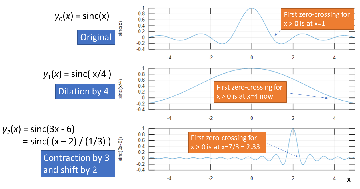
Figure 1.8 provides two examples of manipulating the independent variable of the sinc function, which is defined in Appendix A.12. The $sinc$ function is zero when the abscissa $x$ is an integer number $x \in ℤ$ , with the exception of $x = 0$ . Hence, for $x > 0$ , the first zero of $y_{1} (x) = sinc (x ∕ 4)$ is at $x = 4$ . The first zero of the signal $y_{2} (t) = sinc (3 x - 6)$ for $x > 0$ can be found using $3 x - 6 = 1$ , which leads to $x = 7 ∕ 3 \approx 2.33$ , as indicated in Figure 1.8. The contraction and time-shift of $sinc (t)$ is widely used as part of the D/A conversion, as will be discussed in Eq. (3.17).

Figure 1.8: Examples of manipulating the independent variable (in this case $x$ ) of a $sinc$ function.

Example 1.6. Generating graphs of the sinc function. The function sinc in Matlab/Octave can be used to plot a generic sinc with amplitude $A$ , support $ξ$ and centered at $γ$ seconds. The command x = A*sinc((t-gamma)/xi), where t is an array of time instants, provides the amplitude values for the signal

x (t) = A sinc (\frac{t - γ}{ξ}) .

Listing 1.3: MatlabOctaveCodeSnippets/snip_signals_sinc.m. [ Python version]

1Ts = 0.001; %sampling interval (in seconds) 
2xi = 0.2; %support of the sinc in seconds 
3gamma = 0.5; %time shift 
4t = -1.6:Ts:1.6; %define discrete-time abscissa with fine resolution 
5x = 3*sinc((t-gamma)/xi); %define the signal x(t) 
6plot(t,x);

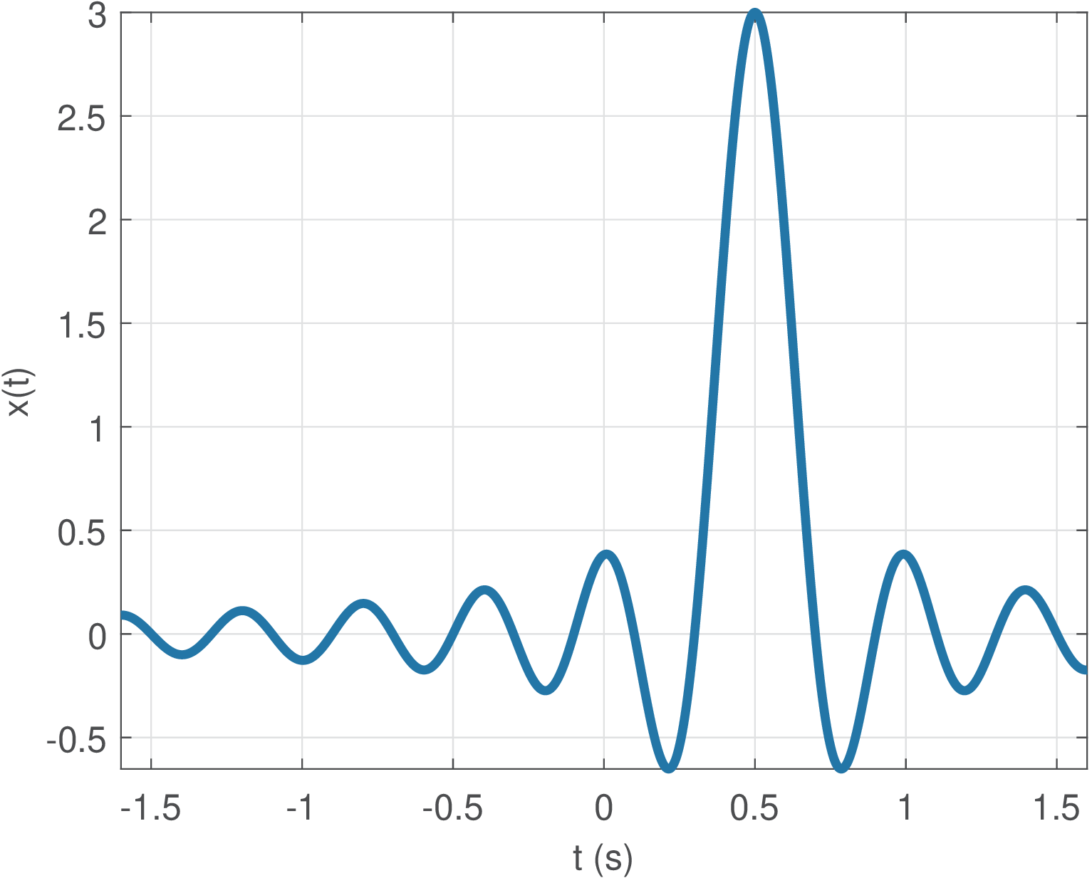
Figure 1.9: Graph of a continuous-time sinc function centered at $t = 0.5$ s, obtained with Listing 1.3.

Listing 1.3 provides an example of using sinc to create a graph of a continuous-time signal sinc, which is depicted in Figure 1.9. The continuous-time sinc in Listing 1.3 corresponds to:

x (t) = 3 sinc (\frac{t - 0.5}{0.2}),

and the chosen sampling interval was $T_{s} = 0.001$ s. We chose a relatively small value for $T_{s}$ to obtain a smooth curve representing a continuous-time signal. $□$

1.3.4 Using impulses to represent signals

If you are not familiar with impulses, please first check Appendix A.26.

Recall that the notation $δ (t - t_{0})$ indicates that a continuous-time impulse occurs at time $t = t_{0}$ . For example, $δ (t - 3)$ is a delayed impulse occurring at $t = 3$ and $δ (t + 2)$ is an anticipated impulse occurring at $t = - 2$ . A similar reasoning applies to the discrete-time $δ [n - n_{0}]$ .

Any discrete-time signal can be conveniently represented by a sum of scaled and shifted impulses. To get the basic idea, consider the following example. An array $[3.0, - 1.3, 2.1, 0, 4.2]$ stores the only non-zero samples of a signal $x [n]$ , with the first element corresponding to time $n = 0$ , the second one to $n = 1$ and so on. How would you write an expression for $x [n]$ without using impulses? A wrong guess would be $x [n] = 3.0 - 1.3 + 2.1 + 0 + 4.2$ because that corresponds to having a constant DC value of $x [n] = 8, \forall n$ . The impulse helps locating the desired amplitude in time. In this example, given that the first sample occurs at $n = 0$ , an expression for $x [n]$ using impulses is $x [n] = 3.0 δ [n] - 1.3 δ [n - 1] + 2.1 δ [n - 2] + 4.2 δ [n - 4]$ . Generalizing, any discrete-time signal can be written as

x [n] = \sum_{n_{0} = - \infty}^{\infty} x [n_{0}] δ [n - n_{0}] .

(1.3)

In our example, $x [n_{0}]$ assumes the values $3.0, - 1.3, 2.1, 0, 4.2$ for $n_{0} = 0, \dots, 4$ , respectively. As explained, writing $x [n] = x [0] + x [1] + x [2] + x [3] + x [4]$ does not lead to the proper result because shifted impulses $δ [n - n_{0}]$ are required to specify the corresponding locations of the amplitudes as they vary over time.

Example 1.7. Revisiting the notation for signals. To complement the discussion in Section 1.2.1, consider interpreting Eq. (1.3) as a single sample at a specific “time” $n = n_{1}$ . To make that clear, one can write:

x [n_{1}] = \sum_{n_{0} = - \infty}^{\infty} x [n_{0}] δ [n_{1} - n_{0}]

(1.4)

and interpret that $δ [n_{1} - n_{0}] = 1$ if $n_{1} = n_{0}$ and zero otherwise. Hence, the summation eliminates all amplitudes of $x [n]$ other than $x [n_{1}]$ , which is the amplitude of $x [n]$ at $n_{1}$ . In this interpretation, Eq. (1.3) and Eq. (1.4) represent a single sample. Alternatively, one can interpret Eq. (1.3) as the whole sequence. Understanding both interpretations is also useful when dealing with continuous-time impulses as discussed in the next paragraph. $□$

The continuous-time version of Eq. (1.3) is

x (t) = \int_{- \infty}^{\infty} x (τ) δ (τ - t) dτ,

(1.5)

which uses the sifting property of impulses (see Appendix A.26) to show that any continuous-time signal $x (t)$ can be represented as a composition of impulses. Besides, similar to to its discrete-time version (Eq. (1.3)), Eq. (1.5) can be interpreted as representing the whole signal or a single sample value at time $t$ .

1.3.5 Using step functions to help representing signals

The continuous-time step function $u (t)$ is defined as 1 for $t > 0$ and 0 for $t < 0$ . There is a discontinuity at $t = 0$ and the amplitude is conveniently assumed to be $u (t) |_{t = 0} = 0.5$ . The discrete-time version $u [n]$ does not have discontinuities and is defined as 1 for $n \geq 0$ and 0 for $n < 0$ . The step function is very useful to indicate signals that are zero for negative values of the independent variable $t$ or $n$ . Another use is to describe finite-duration signals. When a signal ( $x [n]$ or $x (t)$ ) has finite support, it is called a finite-duration signal.

It is easy to represent finite-duration signals using a programming language (Python, Java, C, etc.) or an environment such as Matlab or Octave. The step function can be used with the same goal when dealing with expressions. Say for example that the signal $x [n]$ has only four non-zero samples $[9, 16, 25, 36]$ at $n = 3, 4, 5$ and 6. This signal could be written as $x [n] = n^{2} (u [n - 3] - u [n - 7])$ .

A side note is that $u (t)$ can simplify integrals by limiting the integration interval. For example, $\int_{- \infty}^{\infty} x (t) d t$ when $x (t) = e^{- 2 t} u (t)$ can be obtained by

\int_{- \infty}^{\infty} e^{- 2 t} u (t) d t = \int_{0}^{\infty} e^{- 2 t} d t,

(1.6)

where the role played by $u (t)$ is absorbed by changing the inferior limit to 0. After this step, $u (t)$ can be eliminated from the integral. In other words, when $u (t)$ appears in integrals it can be often taken care of by simply adjusting the integral limits.⁶

1.3.6 The rect function

The rectangular or rect function corresponds to a normalized pulse with unitary support from $t = - 0.5$ to 0.5 and amplitude equals to 1. It can be written as $rect (t) = u (t + 0.5) - u (t - 0.5)$ and in some textbooks it is denoted as $Π (t)$ . The $rect (t)$ is defined here as a continuous-time function, but there are other definitions, for rectangular discrete-time signals.

As an example of a signal derived from $rect (t)$ , consider a pulse $x (t)$ with amplitude $A = 4$ volts and support from 5 to 8 seconds can be denoted as $x (t) = 4 rect ((t - 6.5) ∕ 3)$ . In this case, as explained in Example 1.5, the value $6.5$ is obtained by observing that the intermediate result $rect (t ∕ 3)$ has support (or width) from $t = - 1.5$ to 1.5, and this range must be delayed by 6.5 to obtain the new support as $t = 5$ to 8 s.

Example 1.8. Generating graphs of continuous and discrete-time signals with the rect function. The function rectpuls in Matlab/Octave can be used to plot a generic pulse with amplitude A, support of T and centered at tc seconds. The command x = A*rectpuls(t-tc,T), where t is an array of time instants, provides the amplitude values for the signal

x (t) = A rect (\frac{t - t_{c}}{T}) .

Listing 1.4: MatlabOctaveCodeSnippets/snip_signals_rect.m. [ Python version]

1%% Mimicking a continuous-time signal by using plot 
2Ts = 0.001; %sampling interval in seconds 
3t = -0.8:Ts:0.8; %discrete-time in seconds 
4pulse_width = 0.2; %support of this rect in seconds 
5tc = 0.4; %center (in seconds) of this rect 
6A = 2.5; %amplitude (in Volts) of this rect 
7x = A*rectpuls(t-tc,pulse_width); 
8subplot(211), plot(t,x) %plot as a continuos-time signal 
9xlabel('t'), ylabel('x(t)') 
10%% Making explicit the signal is discrete-time by using stem 
11n = -10:10; %discrete-time in seconds 
12pulse_width = 5; %support of this rect in samples 
13nc = -3; %center (in samples) of this rect 
14A = 7; %amplitude (in Volts) of this rect 
15x = A*rectpuls(n-nc,pulse_width); 
16subplot(212), stem(n,x) %plot as a discrete-time signal 
17xlabel('n'), ylabel('x[n]')

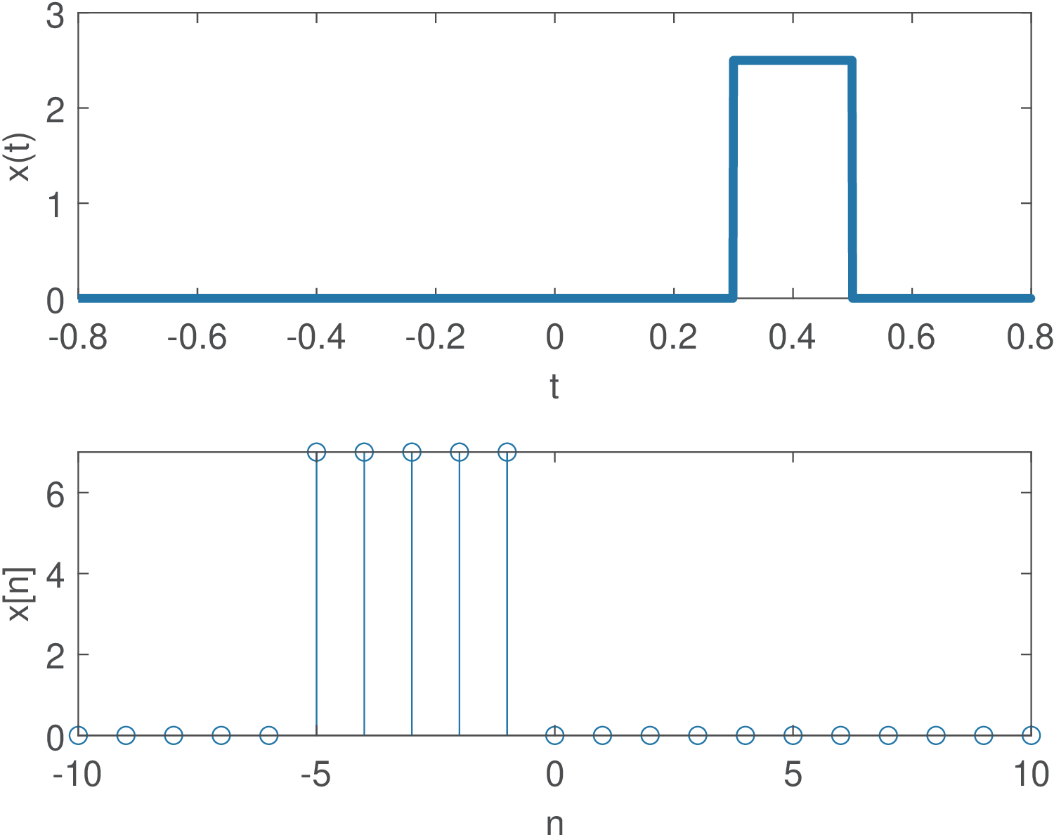
Figure 1.10: Graphs of continuous and discrete-time signals obtained with the rect function in Listing 1.4.

Listing 1.4 provides examples of using rectpuls to create graphs of discrete and continuous-time signals, which are depicted in Figure 1.10. The continuous-time rect in Listing 1.4 corresponds to:

x (t) = 2.5 rect (\frac{t - 0.4}{0.2}) .

One important trick to get a graph that resembles a pulse is to use a small sampling interval, as done in Listing 1.4.

In spite of $rect (t)$ being defined in continuous-time, it is possible to use it to obtain a discrete-time signal as done, e. g., in Listing 1.4. Defining the sampling interval as $T_{s} = 1$ second, allows to create a discretized time axis $n$ composed only by integers, and then generate

x (t) = x [n] = 7 rect (\frac{n + 3}{5}),

with the key assumption of $T_{s} = 1$ . $□$

Example 1.9. Generating a signal composed by several rect functions. The goal in this example is to generate the signal

x (t) = rect (\frac{t}{0.2}) - 3 rect (\frac{t - 0.2}{0.2}) + 3 rect (\frac{t - 0.4}{0.2})

(1.7)

using rectpuls in Matlab/Octave. Listing 1.5 provides a solution, and generates Figure 1.11.

Listing 1.5: MatlabOctaveCodeSnippets/snip_signals_three_rects.m. [ Python version]

1%% Mimicking a continuous-time signal by using plot 
2Ts = 0.001; %sampling interval in seconds 
3t = -1.6:Ts:1.6; %discrete-time in seconds 
4pulse_width = 0.2; %support of this rect in seconds 
5x = rectpuls(t,pulse_width) - 3*rectpuls(t-0.2,pulse_width) + ... 
6    3*rectpuls(t-0.4,pulse_width); %define the signal 
7plot(t,x) %plot as a continuos-time signal 
8xlabel('t'), ylabel('x(t)')

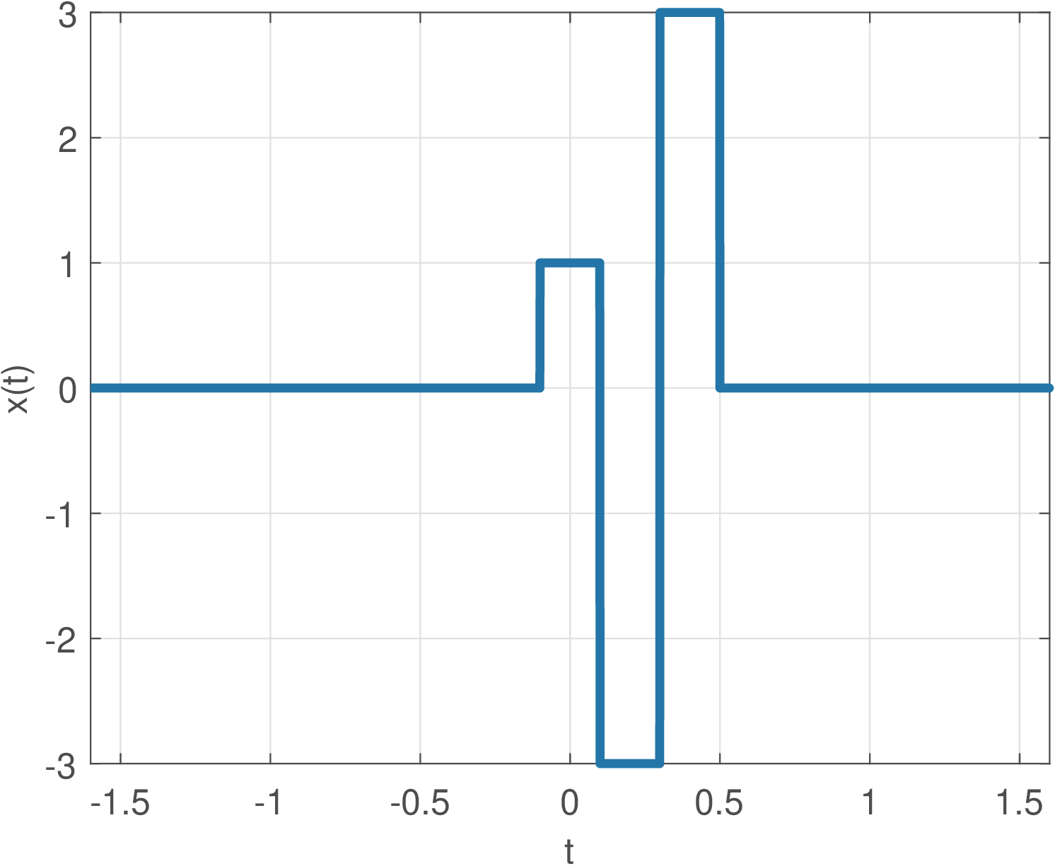
Figure 1.11: Graph of the signal described in Eq. (1.7).

Listing 1.5 illustrates a general procedure: one can define a common time axis $t$ and compose a sophisticated signal $x (t)$ by summing the appropriate parcels. $□$

⁵ The support of a function is the subset ${x : f (x) \neq 0}$ of the function domain that are not mapped to zero. A similar definition can be applied to signals. For instance, the support of a signal $x (t)$ is the set of ranges of $t$ for which $x (t)$ is non-zero.

⁶ There is no need for using, e. g., the integration by parts of Eq. (A.27) to solve Eq. (1.6).