Advanced: Complex-Valued and Sampled Signals

1.5 Advanced: Complex-Valued and Sampled Signals

Some signals are useful for developing theoretical models, even if they do not exist in practice. This section describes two important mathematical representations for signals.

1.5.1 Complex-valued signals

The definition of a signal $x (t)$ (or $x [n]$ ) can be expanded to include complex-valued amplitudes $x (t) \in ℂ$ . In several situations, it is mathematically convenient to use a single complex-valued signal to represent two (typically related) real-valued (or simply real) signals. For instance, the complex-valued exponential $z (t) = e^{j w_{c} t} = cos (w_{c} t) + j sin (w_{c} t)$ (see Euler’s Eq. (A.1)) plays important role in Fourier analysis and simplifies the notation that, otherwise, would rely on two signals: $cos (w_{c} t)$ and $sin (w_{c} t)$ .

A complex-valued signal $x (t) = x_{re} (t) + j x_{im} (t)$ can be interpreted as representing two distinct signals, corresponding to the real $x_{re} (t)$ and imaginary $x_{im} (t)$ components. This representation is widely used in digital communications to compose quadrature signals. In quadrature processing, the component $x_{re} (t)$ is called in-phase and denoted as $x_{i} (t)$ while $x_{im} (t)$ is called the quadrature component and denoted as $x_{q} (t)$ . The quadrature $x_{quadrature} (t)$ signal is real-valued and can be obtained via

x_{quadrature} (t) = x_{i} (t) cos (ω_{c} t) + x_{q} (t) sin (ω_{c} t),

(1.11)

where $ω_{c}$ is a carrier frequency in radians per second. The name quadrature comes from the fact that the sine is a cosine delayed by 90 degrees.

An alternative way of implementing Eq. (1.11) is by defining the complex-valued signal $x_{ce} (t) = x_{i} (t) - j x_{q} (t)$ and using the compact notation

x_{quadrature} (t) = R eal {x_{ce} (t) e^{j ω_{c} t}},

(1.12)

where $R eal {\cdot}$ denotes the real part of a complex-valued signal.

Later (for instance, after transmitting the quadrature signal through a communication channel), the components $x_{i} (t)$ and $x_{q} (t)$ can be recovered from $x_{quadrature} (t)$ . The systems that recover these components typically use quadrature sampling, in which two ADCs deal with the two components $x_{i} (t)$ and $x_{q} (t)$ that may be interpreted as composing a complex-valued signal $x_{ce} (t)$ .

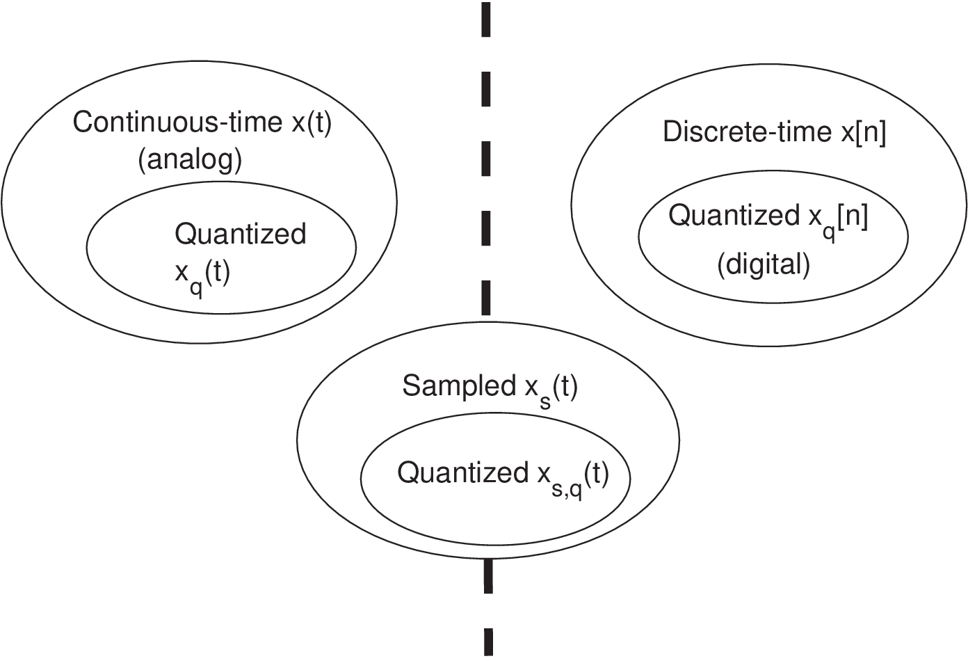
Note that the notation $x_{q} (t)$ is also used for quantized continuous-time signals in Section 1.2, but the context will disambiguate these two categories of signals.

1.5.2 Sampled signals

In a sampled signal $x_{s} (t)$ , the information is represented by uniformly spaced impulses with distinct areas. Because the impulses have undefined (infinite) amplitude values, $x_{s} (t)$ will not be considered here a continuous-time signal, but an intermediate representation between the continuous and discrete-time worlds as indicated in Figure 1.14. Signals other than impulses (e. g., pulses) can be used for sampling, but an impulse train is the only option discussed here due to its mathematical convenience. Assuming impulses, the sampled signal is not physically realizable but it is very useful for mathematically modeling the sampling step of the A/D conversion, as will be discussed in the next paragraphs.

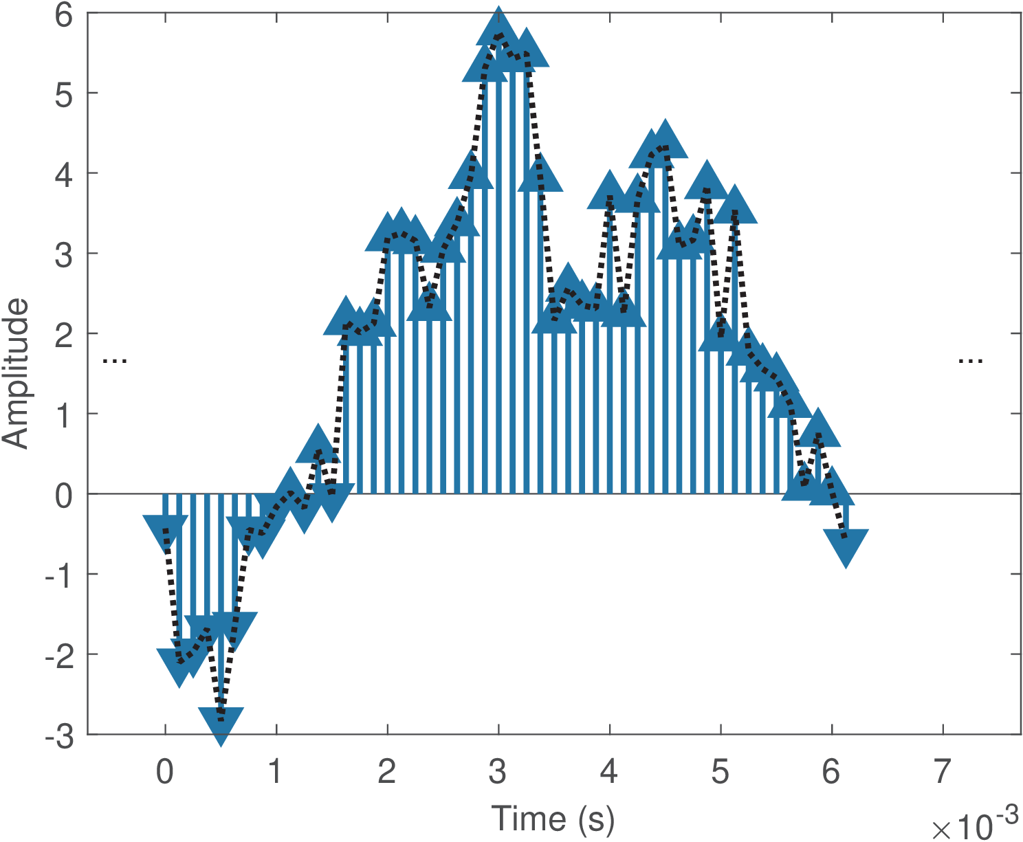
Figure 1.14: Signals classification including the sampled signals.

Figure 1.15: Example of a sampled signal obtained from Figure 1.1. Note the abscissa is continuous but the amplitudes of the impulses go to infinite. Conventionally, the impulse height is used to indicate the impulse area and the contour created by the arrow heads resembles the original analog signal.

In this text, a sampled signal $x_{s} (t)$ is assumed to be the result of periodic sampling a continuous-time signal $x (t)$ . Hence, the sampled signal is composed by periodically spaced impulses whose areas correspond to the value of the original analog signal $x (t)$ at the impulse location. There is a convention for showing plots of sampled signals with the impulse heights corresponding to their areas (see Appendix A.26), but the infinite amplitude of $x_{s} (t)$ is considered $\pm \infty$ at the impulses positions. The amplitude is zero if $t$ is not a multiple of $T_{s}$ , i. e., $x (t) = 0, \forall t \neq k T_{s}$ , where $k \in ℤ$ is any integer.⁷

Figure 1.15 presents an example of a sampled signal. It can be compared with Figure 1.1 and Figure 1.2. Figure 1.15 was obtained assuming the time interval between consecutive impulses is $T_{s} = 125$ $μ$ s (or, equivalently, that $F_{s} = 1 ∕ T_{s} = 8$ kHz). Note also that the sampled signal $x_{s} (t)$ in Figure 1.15 exists for all $t$ , while a discrete-time signal $x [n]$ is considered to exist only for $n \in ℤ$ . Another distinction is that $t$ in $x_{s} (t)$ (as well as in $x (t)$ ) has dimension of time (assumed to be in seconds) while $n$ in $x [n]$ is dimensionless.

⁷ A signal $z (t)$ that contain impulses $δ (t)$ but is not obtained via periodic sampling, will not be denoted with the subscript $s$ nor considered a sampled signal.