4.3 Windows for spectral analysis
Windows were briefly discussed in the context of block processing and FIR design in Sections 1.4 and 3.14.5, respectively. Here they are applied to spectral analysis in order to better control trade offs such as resolution and leakage.
Windows are essential to model1 the extraction of a finite-duration segment from a signal with a potentially infinite duration. For example, a -point FFT is restricted to operate on signal samples, with . And even if the user is not aware or explicitly modeling the windowing operation, obtaining a segment of samples from an eventually longer signal is mathematically equivalent to multiplying by a rectangular window of duration samples (as implicitly done in Section 1.4).
This windowing operation in time domain can often be modeled by
|
| (4.1) |
as a pre-processing step, to generate with a finite duration of samples. Windowing enables calculating the FFT of the finite-duration , while the FFT of the original signal would be unfeasible due to its long duration.
As informed by Eq. (3.10), this multiplication in time-domain corresponds to a periodic convolution in frequency-domain, as repeated here for convenience:
|
| (4.2) |
between the DTFTs and of and , respectively.
Five popular windows are discussed in the next subsection.
4.3.1 Popular windows
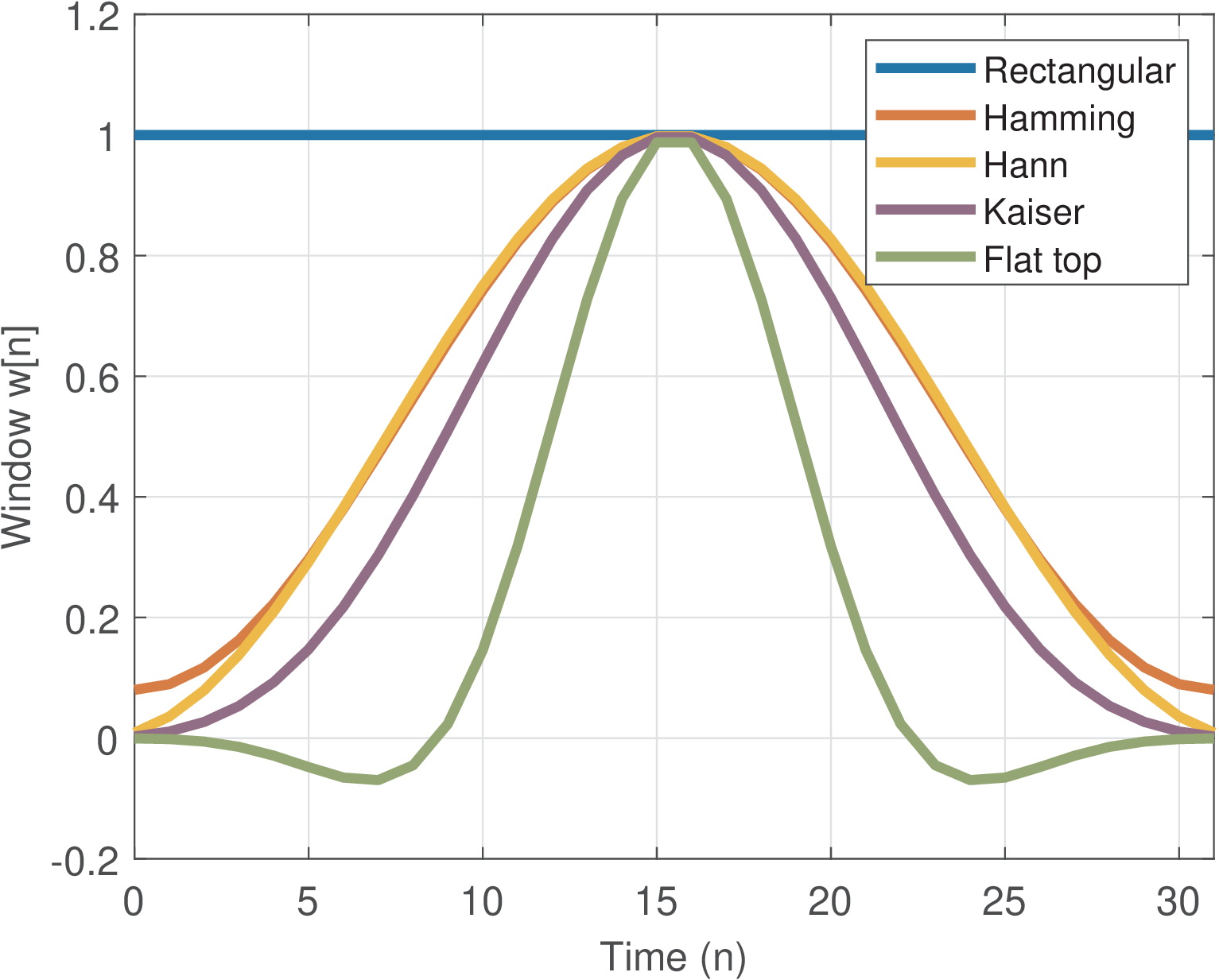
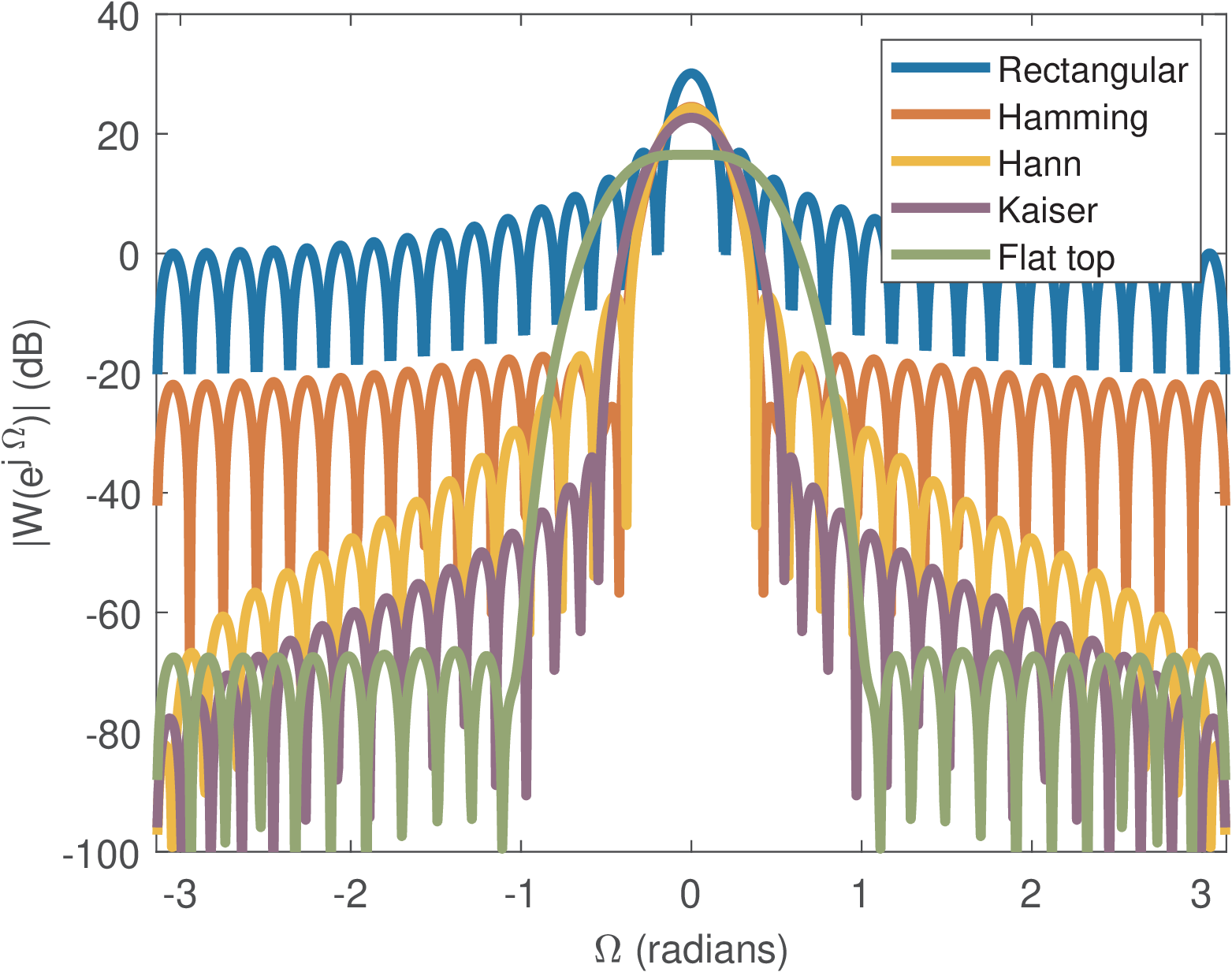
Figure 4.1 shows some common windows for the case of samples in time-domain. Note that all of them were normalized to have the maximum amplitudes equal to one. Figure 4.2 shows these windows in frequency-domain, via their DTFTs.
Example 4.1. Designing windows in Matlab/Octave. Listing 4.1 lists the commands to design windows with samples using Matlab/Octave.
1N=256; %desired number of samples of window W
2W=rectwin(N); %Rectangular window
3W=hamming(N); %Hamming window
4W=hanning(N); %Hann window
5W=kaiser(N,7.85); %Kaiser with beta=7.85
6W=flattopwin(N); %Flat top window
Assuming discrete-time windows, the only input parameter for their design is their duration N. The Kaiser windows (also called Kaiser-Bessel window) is the only exception among the five, because it also has a parameter . For example, increasing of a Kaiser window widens the main lobe and decreases the amplitude of the sidelobes.
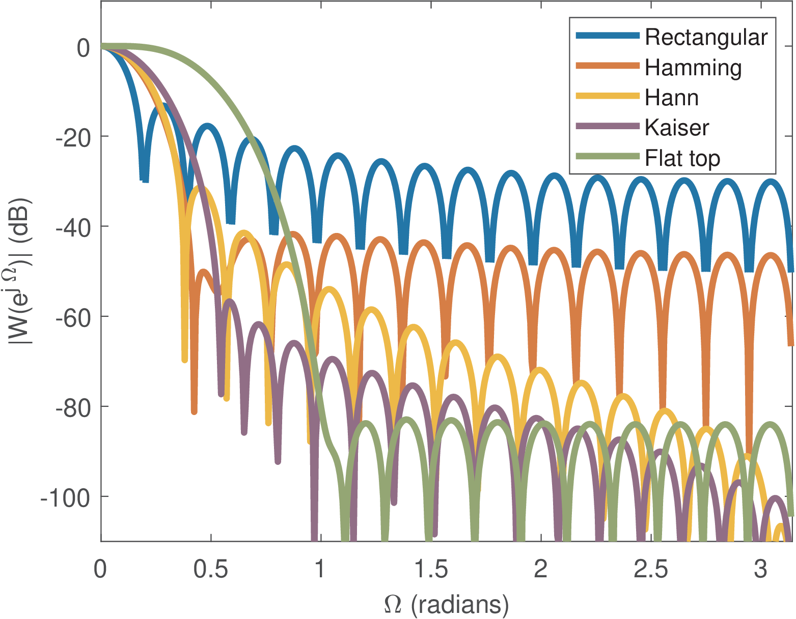
It is common to normalize a window such that its DTFT has a value equal to one at DC. This was done to generate Figure 4.3. To obtain this normalization, one can use the fact that the DC value , where is the Z transform of the window , coincides with the sum of the window coefficients. For example, a normalized Hamming window can be obtained with w=hamming(32);w=w/sum(w).
Equations describing popular windows
The Hamming window adopted here is given by
|
| (4.3) |
|
| (4.4) |
Note that according to Eq. (4.4), the first and last samples ( and ) are zero and this version of the Hann window is called “periodic”. In Python, the commands import numpy and w = numpy.hanning(5) return [0.,0.5,1.,0.5,0.]. In Matlab/Octave, the command hanning(6,’periodic’) returns [0;0.25;0.75;1.00;0.75;0.25] while the commands hanning(5) and hanning(5,’symmetric’) return [0.25;0.75;1.00;0.75;0.25], without the zero-valued samples.
The Kaiser windows for odd, such that is an integer, is
|
| (4.6) |
where is the order Bessel function of the first kind, which is calculated in Matlab/Octave with besseli(0,x), as indicated in the following commands:
1N=13; beta=7.85; %produce same window as w=kaiser(N,beta):
2n=0:N-1; M=(N-1)/2; %auxiliary variables
3w=abs(besseli(0,beta*sqrt(1-((n-M)/M).^2)))/abs(besseli(0,beta));
4w=w/max(w); %normalize to have maximum value equal to 1
that create a Kaiser window (for odd).
4.3.2 Figures of merit applied to windows
Four of the most important figures of merit (or performance metrics) of a window are:
- width of its main lobe,
- amplitude of its sidelobes,
- rate of sidelobe decay as frequency increases,
- and scalloping loss.
There are other figures of merit of windows, and the reader is invited to check the references about windows in Section 4.13.
Windows differ in their main lobe width, which is typically inversely proportional to , the length of the window. Thus, it is possible to achieve a better resolution in frequency by increasing , but more signal samples are needed and sometimes they are not available.
Another important window parameter is the highest sidelobe level, which should have a small value. When a window is used for FIR design, the smaller the sidelobe amplitude with respect to the amplitude of the main lobe, the higher the filter attenuation in the stopband.
From the spectra in Figure 4.3, Table 4.1 can be obtained, which indicates the difference in dB between the main lobe and the highest sidelobe amplitudes. It should be noticed that, for the Hamming window, the highest sidelobe is the third one. The first sidelobe is localized in the frequency equal to 0.46 rad and has a level of dB when compared to the main-lobe level.
| Window | Rectangular | Hann | Hamming | Kaiser () | Flat top |
| Difference (dB) | |||||
Step 3 in Figure 3.49 illustrates an example of the impact in windows-based FIR design of the main lobe width and the amplitudes of the windows sidelobes. The main lobe of the windows DTFT dictates the transition band and the amplitude of its sidelobes determine the ripples (attenuation values) at the stopband.
When comparing spectral components that are close to each other, the adopted windows must have good resolution and a low highest sidelobe level. When the spectral components are far apart, having a large sidelobe decay (or fall-off) can be more important.
This sidelobe fall-off indicates how the peak amplitude of the sidelobes decay with frequency and, for example, is a motivation for using the Hann window. The side-lobe fall-off is dependent on the continuity of the window in time-domain and its derivatives. For example, the Hann window is continuous, and besides, its first derivative is continuous too. Thus, its transform falls off at or, equivalently, at dB per octave. In contrast, the rectangular and Hamming windows, which are not continuous at their endpoints, have a dB per octave fall-off.
To study windowing, it is useful to know how to locate sinusoids with respect to the frequency grid imposed by the FFT. This is the topic of the following subsection.
Positioning sinusoids with respect to the FFT bin
Given that the bin width of an -point DFT (or FFT) is radians, the angular frequency associated to the -th FFT bin is radians, as given by Eq. (2.40). At this point, it may be useful to recall the definition of a bin center using Figure 2.18.
When performing the spectral analysis of a bin-centered sinusoid using an -point FFT, the components of “positive” and “negative” frequencies of will be mapped to the FFT bins and , respectively. In order to investigate non-bin-centered sinusoids, it is useful to generalize the signal expression to
|
| (4.7) |
where is a real number in the range that allows to obtain any desired value for the positive angular frequency , from 0 to rad.
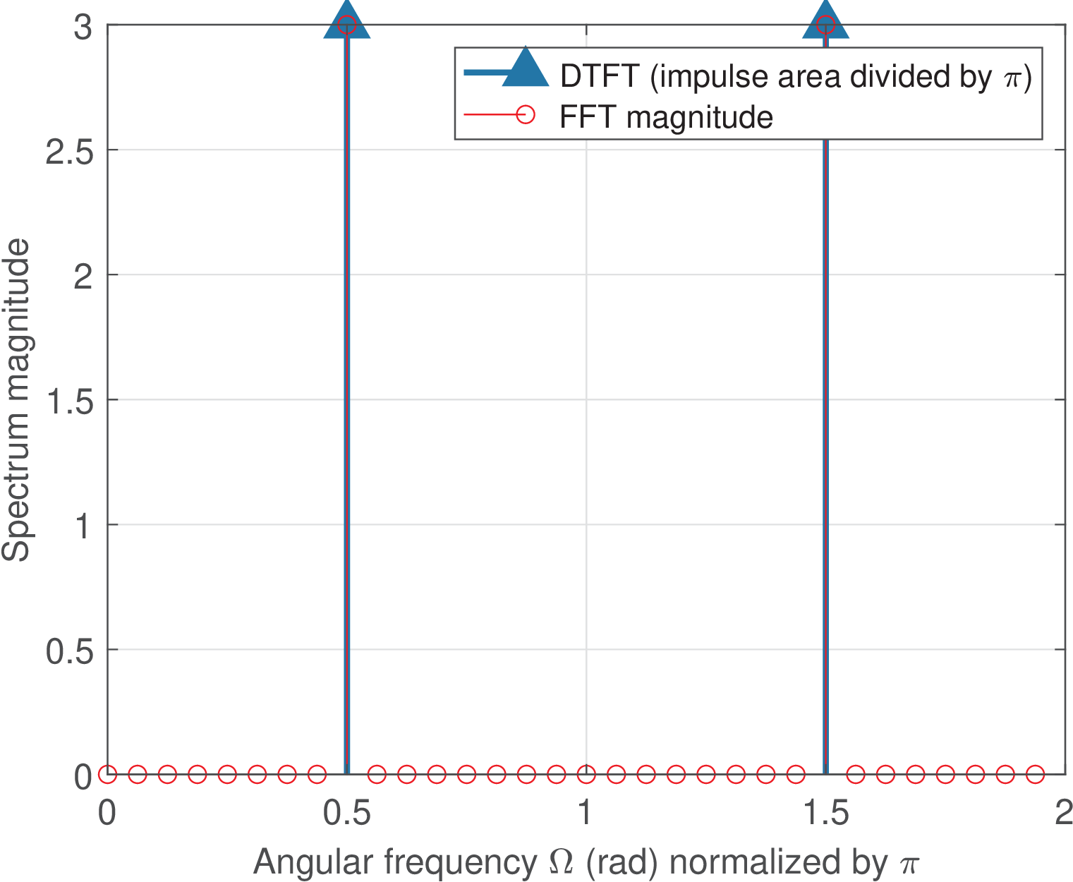
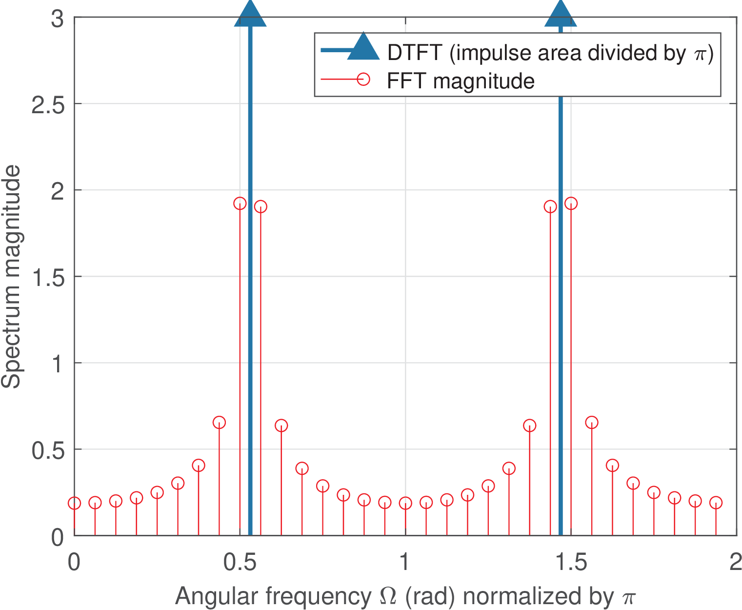
For instance, and , indicates a sinusoid with frequency rad, which corresponds to a bin-centered sinusoid located at the centers of FFT bins (the ninth bin) and bin (negative frequency). This is illustrated in Figure 4.4, where the DTFT of as an infinite-length (eternal) sinusoid of amplitude V is depicted, together with its points FFT magnitude.
As another example, and , indicates the sinusoid now with frequency rad, which is located at the edge between bins and , and at the edge between bins and . This is illustrated in Figure 4.5.
Alternatively, one can write Eq. (4.7) in terms of the FFT resolution as:
|
| (4.8) |
Creating sinusoids according to Eq. (4.7) allows to present the scalloping loss in the subsequent discussion.
Estimating sinusoid amplitude and observing the scalloping loss
In some applications of FFT-based spectral analysis it is necessary not only detect the frequencies (their values in Hertz, for instance) but also the amplitudes (e. g., in volts) of the detected frequency components. In this case, the impact of windowing and then using an FFT needs to be taken in account because they impose an error (called “scalloping” loss) on the estimated sinusoid amplitude with respect to the true value. For most windows, the scalloping loss is worst when the frequency is at the boundary of two neighboring bins (half-way their bin centers).
If one is calculating the harmonic distortion solely based on percentage values, such as: “- the third harmonic has 12% of the amplitude of the fundamental frequency component”, then mitigating the scalloping loss may not be needed. But if the analysis requires the absolute amplitude values of the harmonic components, the scalloping loss issue becomes important.
Listing 4.2 illustrates a procedure for estimating the amplitude V of a cosine using FFT and the effect of the scalloping loss.
1window_choice = 1; %choose one among 3 possible windows
2alpha=8.5; %specifies the cosine frequency
3clf, N=32; A=6; %clear figure, FFT length, cosine amplitude
4Wc=(alpha*2*pi)/N; %cosine frequency in radians
5n=0:N-1; x=A*cos(Wc*n); %generate N samples of the cosine
6switch (window_choice)
7  case 1
8    this_window = rectwin(N);
9  case 2
10    this_window = hanning(N);
11  case 3
12  this_window = flattopwin(N);
13end
14amplitude_scaling = sum(this_window); %factor to mitigate scalloping
15xw = x.* transpose(this_window); %multiply in time-domain
16Xw_scaled_fft = fft(xw)/amplitude_scaling; %N-points FFT and scale it
17max_fft_amplitude = max(abs(Xw_scaled_fft));
18disp(['Max(abs(scaled FFT)) = ' num2str(max_fft_amplitude )])
19scalloping_loss=(A/2)-max_fft_amplitude;
20disp(['Scalloping loss = ' num2str(scalloping_loss)])
21disp(['Correct amplitude (Volts) = ' num2str(A)])
22disp(['Estimated amplitude (Volts) = ' num2str(2*max_fft_amplitude)])
23amplitude_error = A - 2*max_fft_amplitude;
24disp(['Amplitude error (Volts) = ' num2str(amplitude_error)])
25disp(['Amplitude error (%) = ' num2str(100*amplitude_error/A)])
26ak_impulseplot([A/2, A/2],[Wc,2*pi-Wc]/pi,[]); %plot cosine impulses
27hold on, stem([0:N-1]*(2*pi/N)/pi,abs(Xw_scaled_fft),'or')
28xlabel('Angular frequency \Omega (rad) normalized by \pi')
29ylabel('Spectrum magnitude'), grid
30legend('DTFT (impulse area divided by \pi)', 'FFT magnitude')
When Listing 4.2 is used with to generate a bin-centered cosine, the result using the rectangular window is Figure 4.4. Changing the window to flattop leads to Figure 4.6.
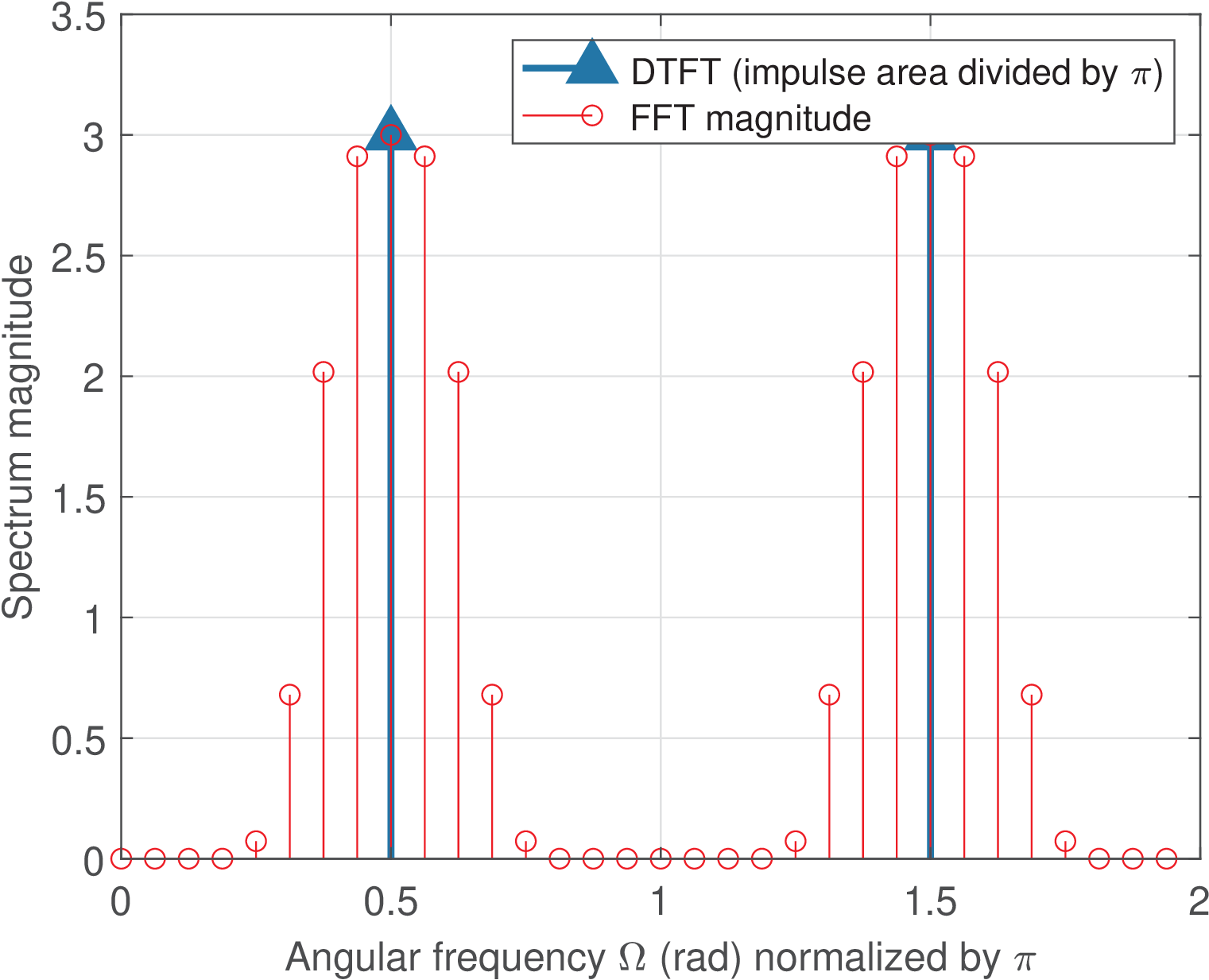
Both Figure 4.4 and Figure 4.6 show that the maximum value of the FFT magnitude, when normalized by the FFT size , leads to the correct amplitude value. In this case of bin-centered sinusoids there is no visible scalloping loss.
However, if the cosine frequency is positioned at the boundary between two neighboring bins (alpha=8.5), the scalloping loss becomes evident. When using the rectangular window with alpha=8.5, one obtains Figure 4.5 and the numerical results below:
Max(abs(scaled FFT)) = 1.9221
Scalloping loss = 1.0779
Correct amplitude (volts) = 6
Estimated amplitude (volts) = 3.8442
Amplitude error (volts) = 2.1558
Amplitude error (%) = 35.9301
The amplitude error in this case is 35.9%, which is due to the worst-case scalloping loss for the rectangular window in this situation of a sinusoid exactly half-way the bins.2
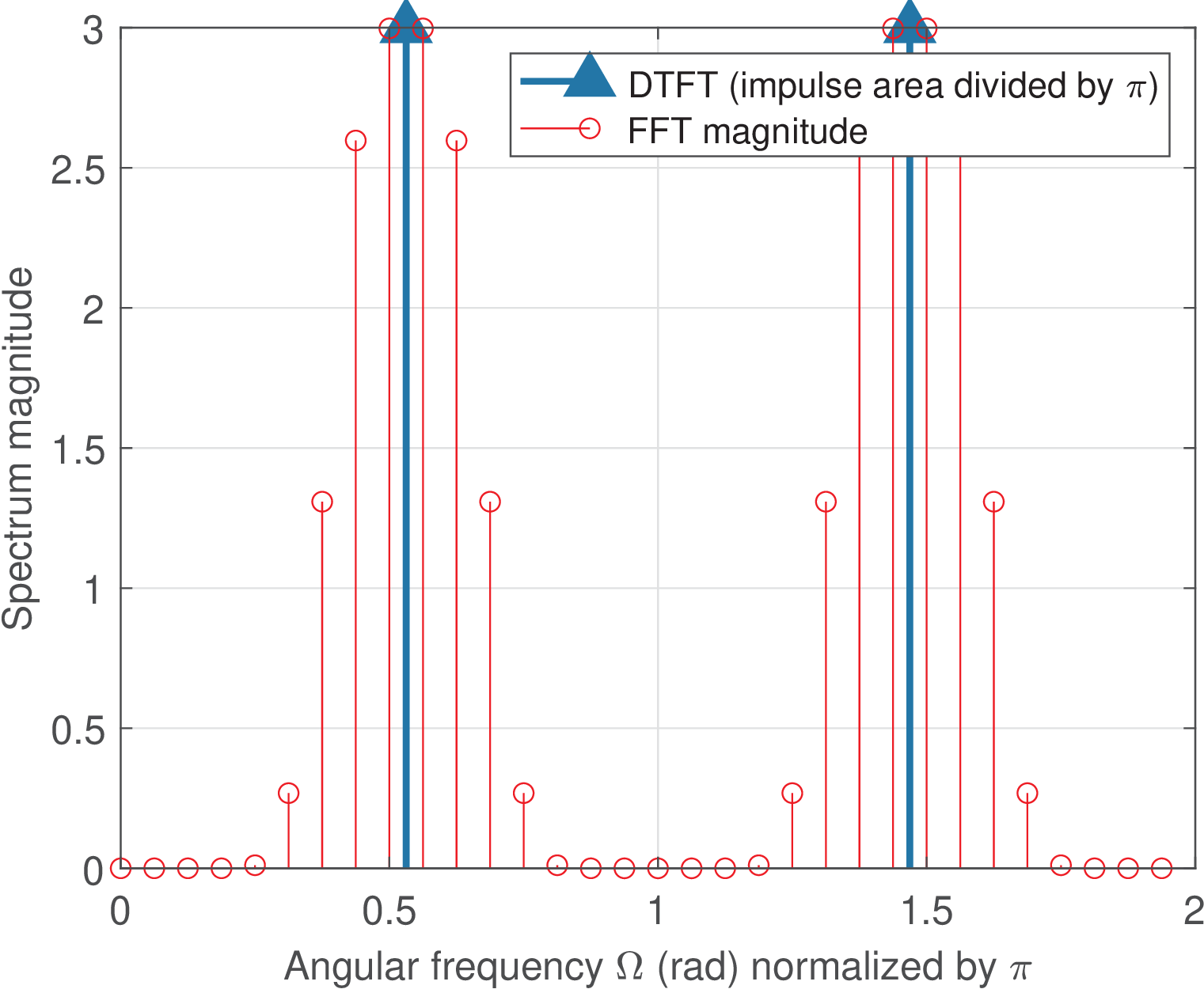
In case one chooses the flat-top window in Listing 4.2 (window_choice=3), the corresponding figure is Figure 4.7 and the numerical results are:
Max(abs(scaled FFT)) = 2.9949
Scalloping loss = 0.0050728
Correct amplitude (volts) = 6
Estimated amplitude (volts) = 5.9899
Amplitude error (volts) = 0.010146
Amplitude error (%) = 0.16909
The flat-top window does not have a good frequency resolution but reaches an amplitude estimation error of only 0.17%. Because of that, it is widely adopt to calibrate equipment.3
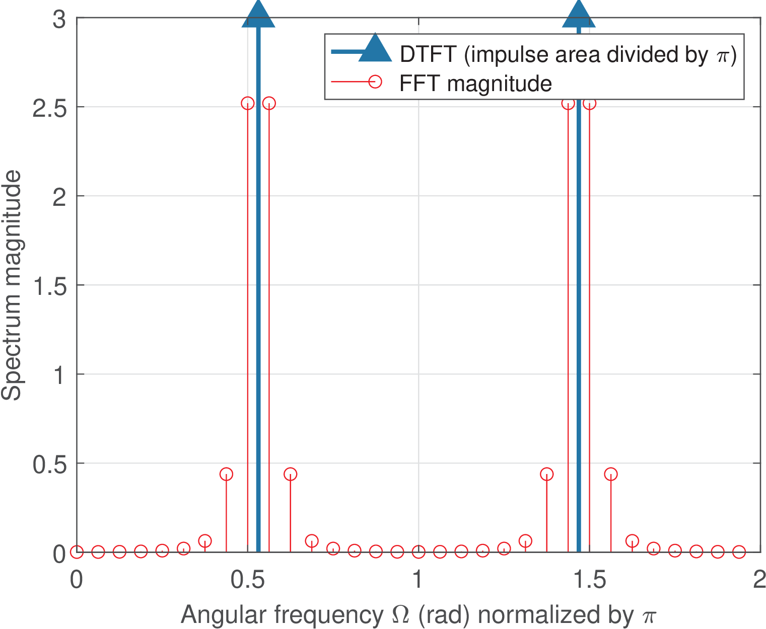
As indicated in Figure 4.8, the Hann window is a trade-off between frequency resolution and amplitude error, reaching 16% of amplitude error when one uses window_choice=2 in Listing 4.2, as listed:
Max(abs(scaled FFT)) = 2.5197
Scalloping loss = 0.48034
Correct amplitude (volts) = 6
Estimated amplitude (volts) = 5.0393
Amplitude error (volts) = 0.96069
Amplitude error (%) = 16.0115
This study just showed the concept of scalloping loss and the importance of choosing the proper window function (such as flattop). A better interpretation of scalloping loss is obtained by interpreting the FFT as a filter bank, as briefly discussed in the next subsection.
Advanced: FFT Interpreted as a Filter Bank
Filter banks are often used for performing spectrum analysis and signal synthesis. A DFT can be seen as a uniform filter bank due to the fact that all filters have the same bandwidth.
The interpretation of FFT and other transforms as filter banks lead to improved insight. For example, the good result obtained by the rectangular window in Figure 4.21 is due to a particular property of its side-lobe structure: all side-lobes are zero in the center of the bins. When the spectrum being analyzed has non-zero components only in bin centers, the leakage due to the side-lobes will not appear in the final FFT result. The leakage could be seen in the DTFT though.
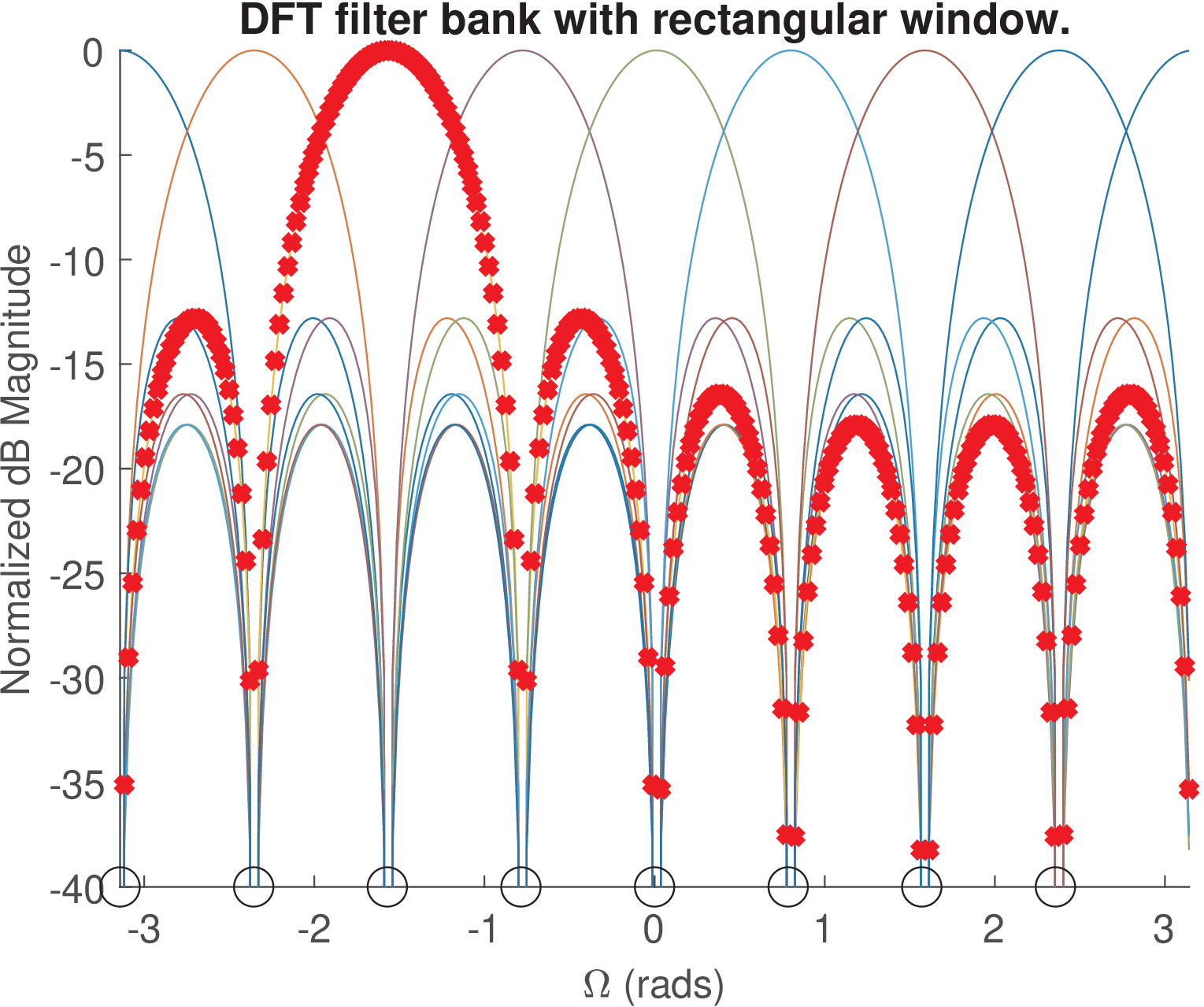
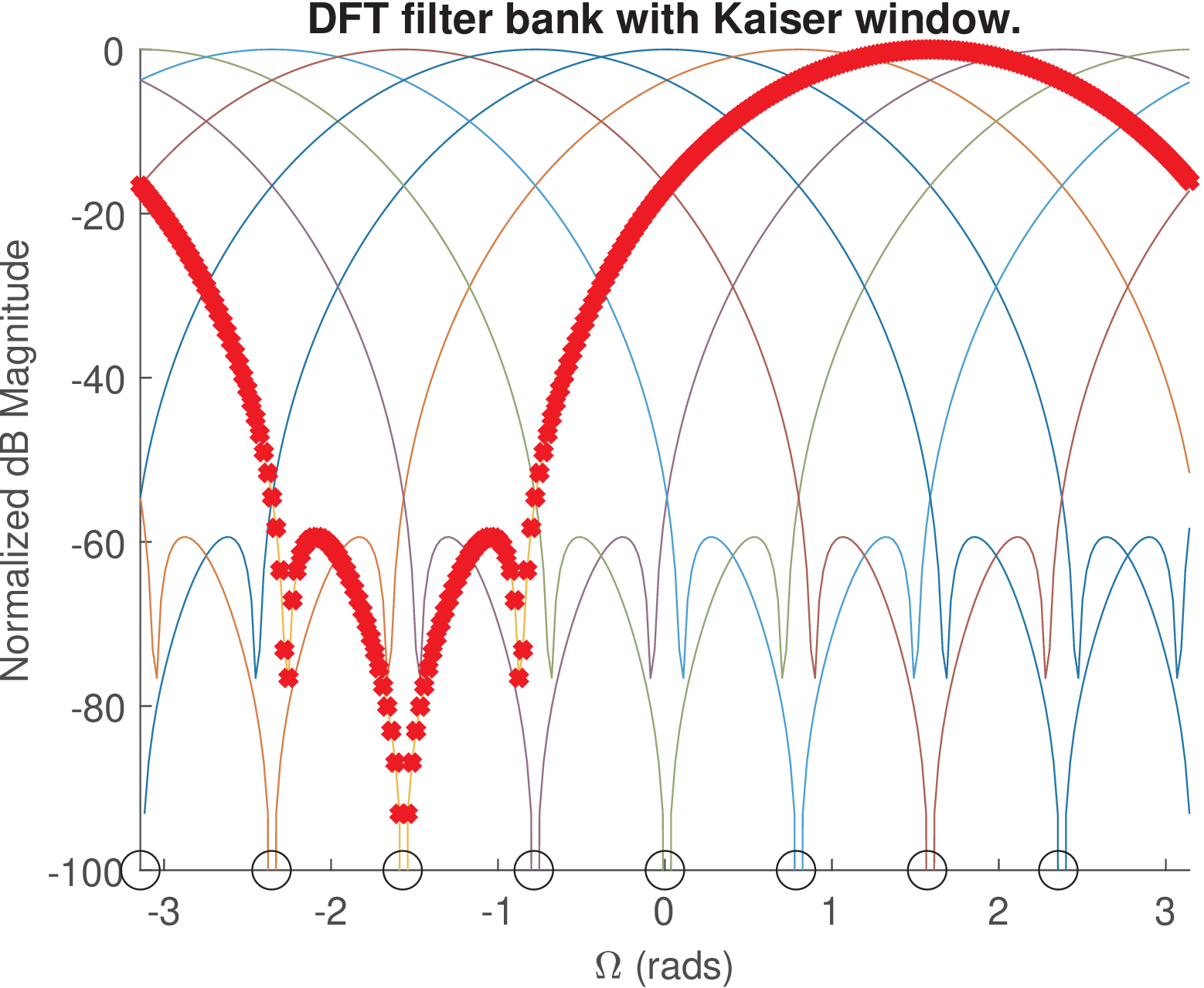
Figure 4.10 and Figure 4.9 indicate the filter banks corresponding to an FFT with rectangular and Kaiser windows, respectively. The rectangular has larger side-lobe levels, but all of them achieve a zero in the bin centers. The Kaiser window does not have side-lobes with amplitude equal to zero in the bin centers, but these side-lobe levels are very small. And there are other strategies (see e. g. [Lyo11]) to mitigate the effects of the scalloping loss that complement choosing a good window function.
Advanced: Relation between roots location and spectrum
A window is used to multiply a signal in time-domain, but for the sake of observing its spectrum, it can be interpreted as the impulse response of a FIR filter, which does not have finite poles, only zeros. Under this assumption, there is an interesting relation between the zeros of the windows, and its spectrum .
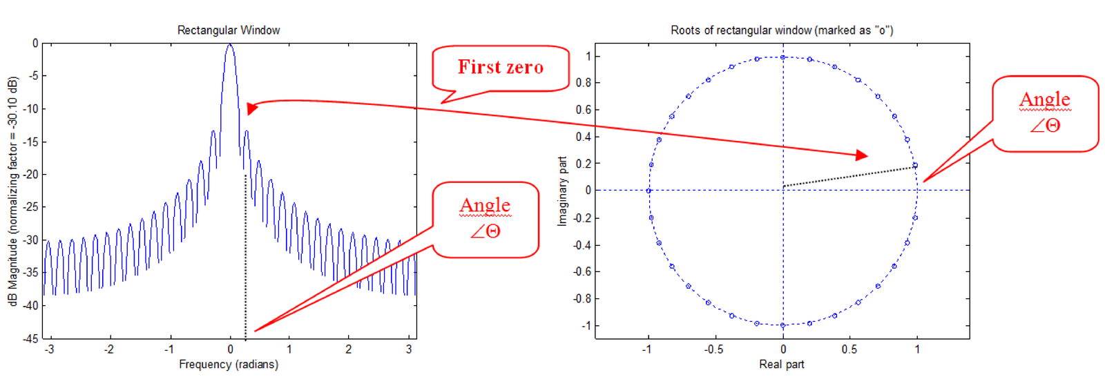
Figure 4.11 shows the spectrum (left plot) of a rectangular window with and the roots (right plot) of this window. This plot outlines that there are zeros (the amount of roots of a polynomial of order ) and the width of the main lobe is obtained from the angle (in this case, rad) of the first root, given that there is no root at and the roots are uniformly spaced around the unit circle.

Figure 4.12 shows that a greater concentration of zeros in the region of the main lobe, allows the Kaiser window (with ) achieve a very small first side-lobe. However, the width of the main lobe increases considerably when compared to the rectangular window in Figure 4.11, due to the increase of . In summary, the rectangular window has the smallest main lobe, but its first sidelobe level is just dB below the main-lobe level. On the other hand, the Kaiser window has a wider main lobe, but this window has very small sidelobe levels.
The next subsections discuss leakage and the picket-fence FFT effect.
4.3.3 Leakage
Leakage is a very important aspect on spectral analysis using FFT. To understand leakage one must remember that the multiplication in time-domain as in Eq. (4.1), corresponds to the convolution in frequency-domain as in Eq. (4.2). The spectra of the windows in Figure 4.2 indicate that the values of the original spectrum will be surely altered if is convolved with any finite-duration window.
The result of the convolution caused by windowing may not significantly impact the original spectrum in case is relatively narrow compared to variations in . But this condition implies that the window is sufficiently long (i. e., must be sufficiently large). As mentioned, the ideal situation, where windowing would not alter the original , is to have as an impulse in the range (i. e. ), but this implies that has infinite duration and all samples of the eventually infinite-length are available for spectral analysis.
Hence, even if is narrow compared to , the convolution may have distinct (“leaked”) values when compared to the original . This is more evident in frequencies where the original signal was zero, and the leakage creates non-zero values in at these frequencies. Step 3 in Figure 3.49 illustrates an example of leakage in windows-based FIR design. The filter frequency response presents “leaked” values (note the ripples) as a result of the (circular) convolution between the DTFTs of the ideal filter and window .
Note that many times, leakage is erroneously interpreted as a consequence of using FFTs to perform spectral analysis. The correct interpretation is that leakage is a consequence of windowing. Even when dealing with DTFTs, without the inherent discretization of frequency provoked by DFTs / FFTs, windowing creates “frequency leaks” that show up on the DTFT . The following paragraphs provide concrete examples of leakage.
Example 4.2. DTFT of a windowed (finite-duration) sinusoid. The DTFT of a finite-duration sinusoid can be obtained by windowing an infinite-length sinusoid . The DTFT of is within the range , then repeated in multiples of .
Assuming a rectangular window with amplitudes equal to 1 from and zero otherwise, the spectrum of as given by Eq. (B.15) is
|
| (4.9) |
The DTFT of the windowed cosine is the periodic convolution between and the window DTFT . Recalling that the periodic convolution of Eq. (4.2) has a factor , the resulting DTFT is
|
| (4.10) |
which can be rewritten as
|
| (4.11) |
Note that the DTFT of a finite-duration sinusoid is very distinct from two impulses (the DTFT of an infinite-length sinusoid) due to the leakage created by windowing.
Example 4.3. Effect of applying finite-length windows (14, 50, and 1000 samples) to an infinite-length sinusoid. Spectrum leakage can be studied by observing the case of the DTFT of a finite-duration sinusoid as given in Eq. (4.11) when the windows duration is 14, 50 or 1000 samples.
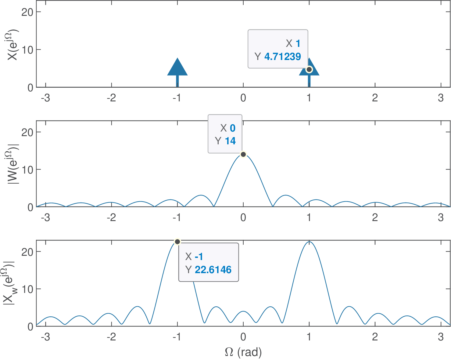
Figure 4.13 depicts the example of an infinite-length cosine with amplitude V and frequency rad, which was then windowed to extract samples. The data tip on the top plot indicates the area of the impulses at is . The middle plot shows and its data tip indicates that its value at DC () is . The bottom plot of Figure 4.13 shows . The value 22.6146 of the data tip at is obtained from Eq. (4.11) as:
The magnitude is the data tip value shown in the bottom plot of Figure 4.13.
As discussed in Section 4.3.2, recovering exactly the amplitude from is not an easy task because the scalloping loss is influenced by contributions from two replicas of in Eq. (4.11).
Figure 4.14 depicts the result when the window length is increased from to samples. In this case, is given by
The magnitude is slightly smaller than , which is the value that would be obtained by using only the first replica of . This uncertainty about the amplitude of the sinusoid provoked by the second replica of can be mitigated using a flattop instead of the rectangular window, as discussed in Section 4.3.2.
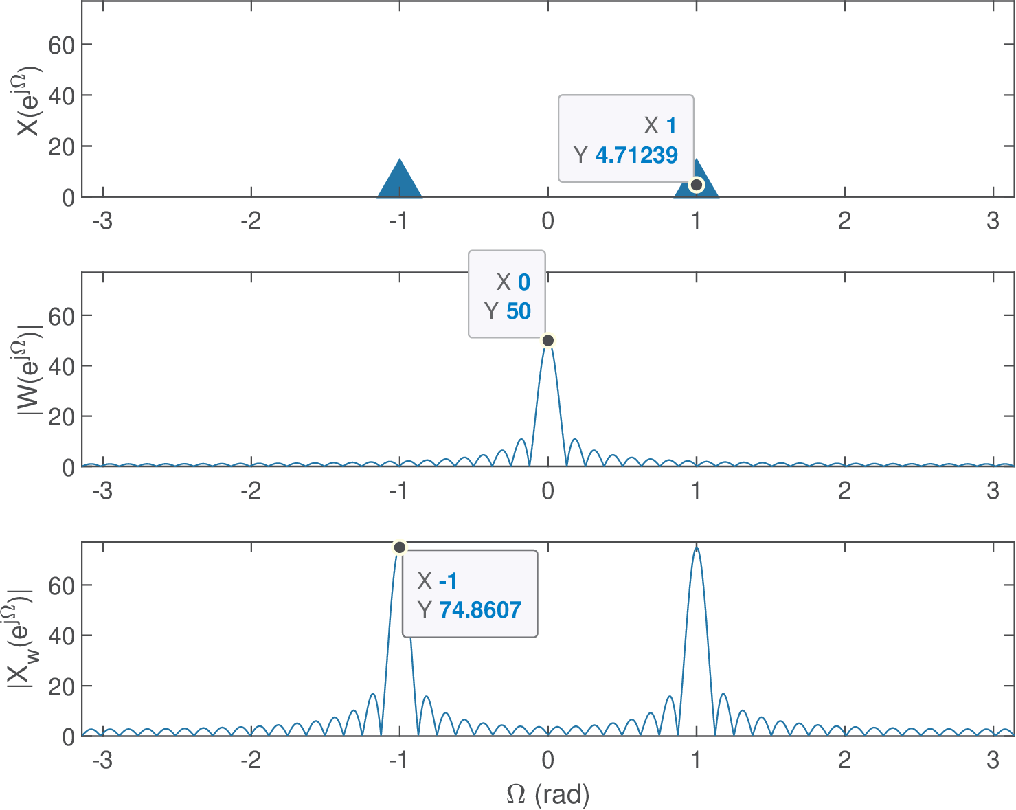
The top plot in Figure 4.13 and Figure 4.14 is showing impulses with the same area values because the input signal does not change, and consequently its DTFT. But the middle plots show that the window DTFT peak gets larger when is increased. Figure 4.15 presents the results when the window length is increased to samples.
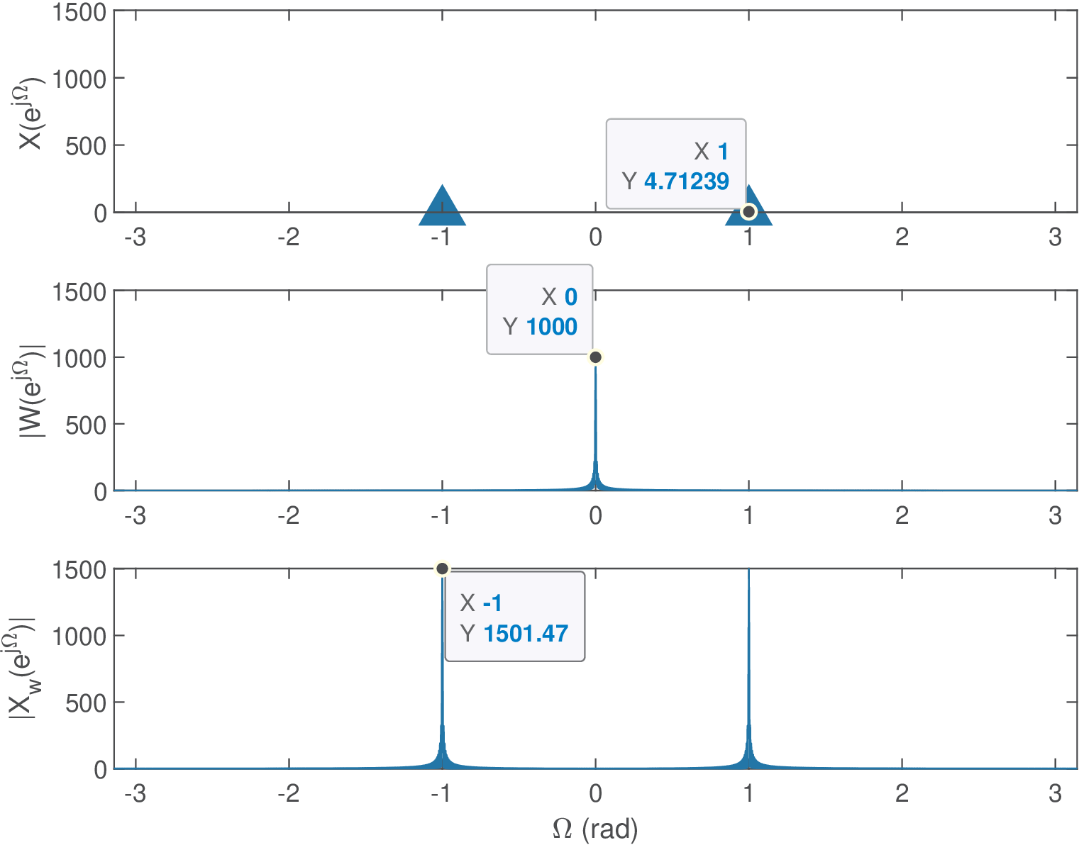
Independent of the window length , a key point made by Figs. 4.13, 4.14 and 4.15 is that the spectrum of a windowed sinusoid is not composed solely of impulses, as in for the infinite-length sinusoid. The DTFT has sidelobes dictated by the window DTFT .
As mentioned, the convolution in Eq. (4.2) may not significantly alter with respect to the original in case is relatively narrow compared to variations in . However, there is a tradeoff between narrower bandwidths and longer duration over time. See, for example, the Fourier transform of a square pulse in Eq. (B.14) to remember the tradeoff between time and frequency. Increasing the duration of (using more samples from the original signal) mitigates leakage as indicated by the behavior of Figure 4.15, which shows the effect of increasing to obtain a window that looks more similar to the ideal impulse.
As previously emphasized, leakage is associated to windowing and should not be confused with the picket-fence effect caused by sampling the DTFT via a FFT, which is discussed in the sequel.
4.3.4 Picket-fence effect
The consequence of discretizing via an FFT is called picket-fence effect. This effect corresponds to observing the DTFT of the signal under analysis just at the DFT/FFT bin centers, as dictated by Eq. (2.40) (or Eq. (2.37), when using frequency in Hz).
It is convenient to interpret FFT-based spectral analysis considering the result of two tasks: 1) windowing a signal and then 2) taking the FFT of the windowed signal. The consequences of each step are, respectively: 1) creation of spectrum with leakage due to windowing, and 2) spectrum values available only at a grid of values imposed by the FFT.
Revisiting scalloping loss as the combined effects of leakage and picket-fence
It is informative to revisit the result of an FFT when the original input signal is a discrete-time sinusoid after windowing, as discussed in Example 4.3.
Recall that the DTFT of the infinite-length cosine is within the range . And the DTFT of the rectangular window is given by Eq. (4.9).
Assuming that denotes the DTFT of the windowed cosine, the final FFT result depends on the two effects:
- f 1.
- Leakage: is the periodic
convolution between
and ,
and is given by Eq. (4.11), which is repeated below for convenience:
- f 2.
- Picket-fence: The FFT has a resolution of and corresponds to samples of the DTFT at frequencies .
Two cases of interest are a bin-centered sinusoid (), and exactly on the boundary of two bins. The latter case represents a worst-case situation with respect to the scalloping loss.
Complementing the experiments in Section 4.3.2, here we study scalloping loss emphasizing the picket-fence effect. For that, one can execute Listing 4.3 with the command snip_frequency_fftCosineExample(8, 2) and snip_frequency_fftCosineExample(8, 2.5) to generate Figure 4.16 and Figure 4.17, respectively. These figures are similar to Figure 4.4 and Figure 4.5. The rectangular window was adopted to generate all four figures. However, it should be noted that the abscissa of Figure 4.4 and Figure 4.5 is (negative after positive frequencies) while Figure 4.16 and Figure 4.17 were obtained with fftshift such that the left-most bins have negative indices .
1function snip_frequency_fftCosineExample(N, alpha)
2% function snip_frequency_fftCosineExample(alpha)
3% Superimposes the DTFT and FFT of a windowed cosine,
4% assuming the rectangular window.
5% N     - FFT length
6% alpha - specifies the cosine angular frequency Wc as
7%         Wc=(alpha*2*pi)/Nfft, where Wc is in radians
8A=6; %cosine amplitude
9if alpha > N/2
10    error('alpha cannot be larger than N/2')
11end
12Wc=(alpha*2*pi)/N; %cosine frequency in radians
13%% Calculate DTFT values in a fine grid
14M=1000; %number of sample points for DTFT visualization
15% discretize the frequency axis in large number M of points:
16Omega = linspace(-pi, pi, M);
17%add frequency values of interest to facilitate plots
18Omega = sort([Omega -Wc Wc 0]);
19Xw = (A/2)*(rect_dtft(Omega+Wc,N) + rect_dtft(Omega-Wc,N)); %DTFT
20%% Calculate DFT
21n=0:N-1; x=A*cos(Wc*n); %generate N samples of the cosine
22Xfft = fftshift(fft(x)); %calculate FFT with N points and shift
23deltaW = 2*pi/N;  %the unit circle was divided in N slices
24if rem(N,2) == 0
25    W_fft = -pi:deltaW:pi-deltaW; %N is even
26else
27    W_fft = -pi+(deltaW/2):deltaW:pi-(deltaW/2); %N is odd
28end
29%% Plot and calculate scalloping loss
30plot(Omega,abs(Xw)),hold on, stem(W_fft,abs(Xfft),'or')
31xlabel('Angular frequency \Omega (rad)')
32ylabel('|X_w(e^{j\Omega})|'), legend('DTFT','DFT')
33grid, axis tight
34disp(['Max(abs(FFT))=' num2str(max(abs(Xfft)))])
35disp(['Scalloping loss in DTFT=' num2str(A*N/2-max(abs(Xfft)))])
36end
37function rect_window_dtft = rect_dtft(Omega, N)
38    %DTFT of rectangular window
39    W_div_2 = Omega/2; %half of angles (pre-compute to speed up)
40    rect_window_dtft=(sin(N*W_div_2)./sin(W_div_2)).*exp(-1j*W_div_2*(N-1));
41    %Use L'Hospital rule to correct NaN if 0/0:
42    rect_window_dtft(isnan(rect_window_dtft))=N;
43end
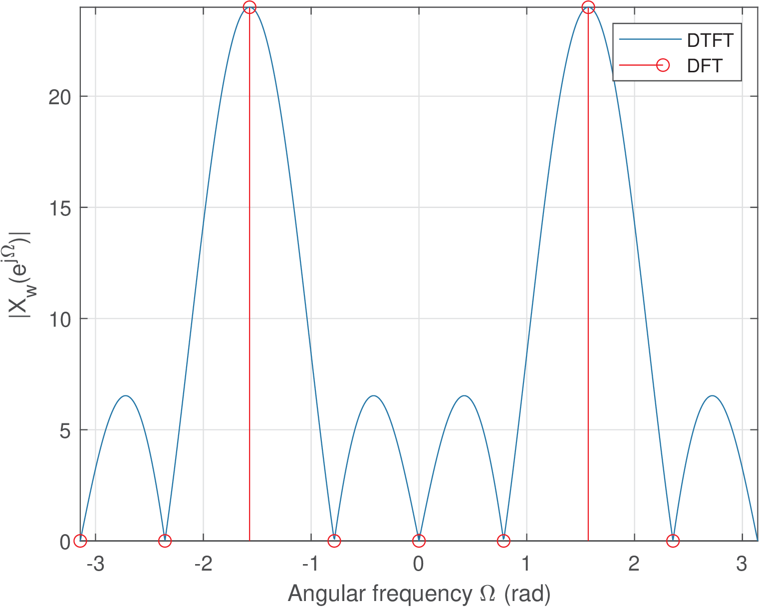
Figure 4.16 indicates that when the sinusoid is bin-centered, the FFT outputs two peaks of value A*N/2, which in this example corresponds to 6*8/2=24. In this case, the scalloping loss is zero and there is no visible leakage. This situation is interesting because as can be observed by the DTFT plot in Figure 4.16, the windowing operation already created leakage, but the picket-fence effect makes it not visible to the user that is observing solely the FFT result , not the DTFT .
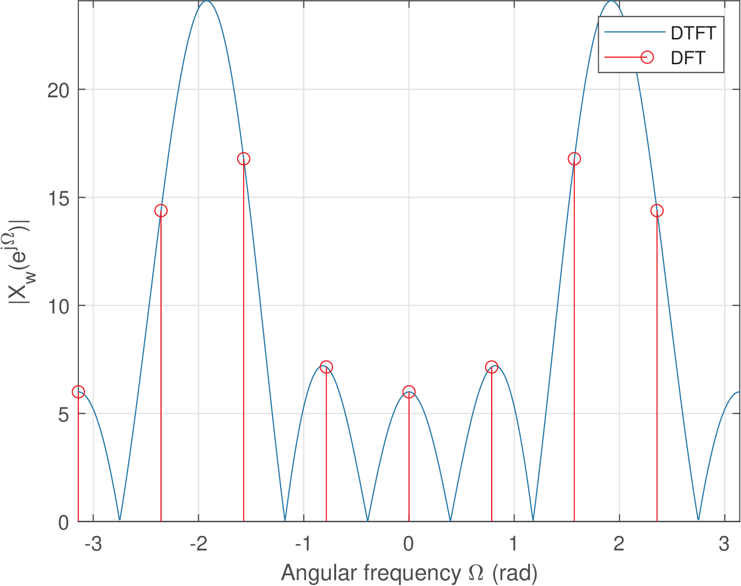
In contrast to Figure 4.16, in Figure 4.17 the picket-fence effect on a non-bin-centered sinusoid clearly discloses an extreme leakage. The adopted value , places the cosine right in the shared edge of bin centers and . The FFT value for is slightly larger () than the value for () due to the influence of the first replica of positioned at rad. In this example, the scalloping loss is calculated with
1disp(['Max(abs(FFT))=' num2str(max(abs(Xfft)))])
2disp(['Scalloping loss in DTFT=' num2str(A*N/2-max(abs(Xfft)))])
and the result is
In this case, the expected (ideal) DTFT peak for the sinusoid with amplitude A=6 would be A*N/2=24, but the maximum of the amplitude spectrum is 16.7876. Hence, the scalloping loss is .
If one uses the fact that should be equal to A*N/2, the sinusoid amplitude can be estimated with V. This corresponds to an error of 1.8031 V with respect to the correct sinusiod amplitude of 6 V.
Advanced: Scalloping loss of sinusoid multiplied by rectangular window
The FFT values of a windowed cosine , with (recall that and ) and assuming a rectangular window, can be obtained by discretizing the frequency axis of Eq. (4.11) to obtain:
|
| (4.12) |
From Eq. (4.9), the value of for rad can be found using L’Hospital’s rule, which leads to .
In the special case of , the signal has a constant amplitude, its DTFT is and the FFT DC bin . This situation is depicted in Figure 4.18.
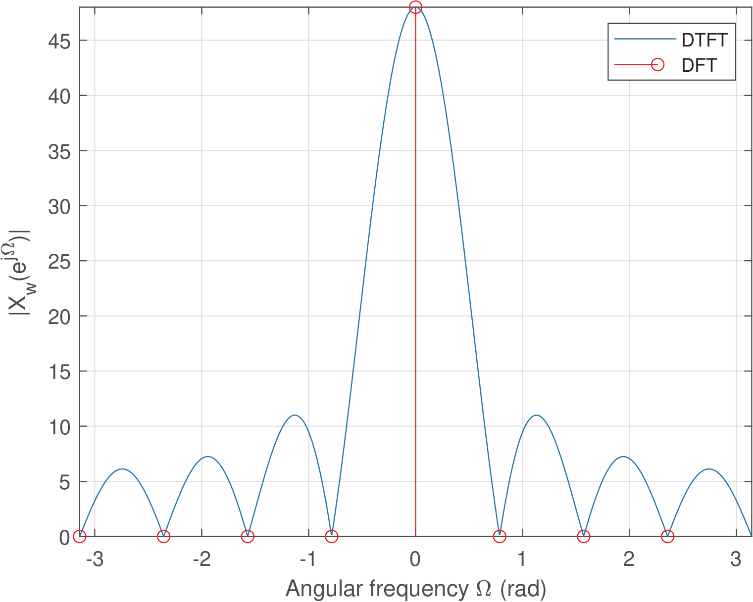
Let us assume the goal is to estimate the sinusoid amplitude in volts, via the DFT coefficients obtained from the signal FFT. In this case, Eq. (2.49), indicates that one needs to normalize the DFT by . Hence, the normalized DC value for Figure 4.18 is . Similarly, when as in Figure 4.16 and Figure 4.17, the two DTFT peaks at have amplitude that lead to an amplitude of for each after division by . In summary, as already discussed in the context of Eq. (2.49), the estimate of amplitudes from a FFT result requires normalizing the absolute values by .
As indicated in Listing 4.3, the scalloping loss for a windowed sinusoid with amplitude when a rectangular window and an -point FFT are used, can be obtained with:
|
| (4.13) |
where is the magnitude corresponding to the FFT bin center that best represents the windowed sinusoid (its strongest FFT component).
4.3.5 Advanced: Only a bin-centered sinusoid leads to an FFT without visible leakage
Leakage and picket-fence make harder to use FFT for analyzing infinite-length sinusoids. In spite of that, the FFT is a flexible tool and its user needs to choose the proper interpretation of its results. For instance, one perspective from the FFT of a windowed signal is that the basis functions of the DFT have a finite duration of samples and can only represent a finite-duration . In this case, the FFT user is not concerned with signal periodicity. Another perspective is to consider that the FFT is estimating the DTFS coefficients and is a single period with samples of a periodic and infinite-length signal. In any case, it is not always possible to conclude about the periodicity and frequency components of the infinite duration by observing only its windowed version .
Recall that, to check the periodicity of , one can use Eq. (1.22) and write
|
| (4.14) |
which is a ratio of two integers when is a rational number (). In case is an integer, then is a rational number. But when and , we still have rational. Hence, can be periodic even if is not an integer. But will be bin-centered, only if is an integer. This is illustrated in the top plots of Figure 4.19.
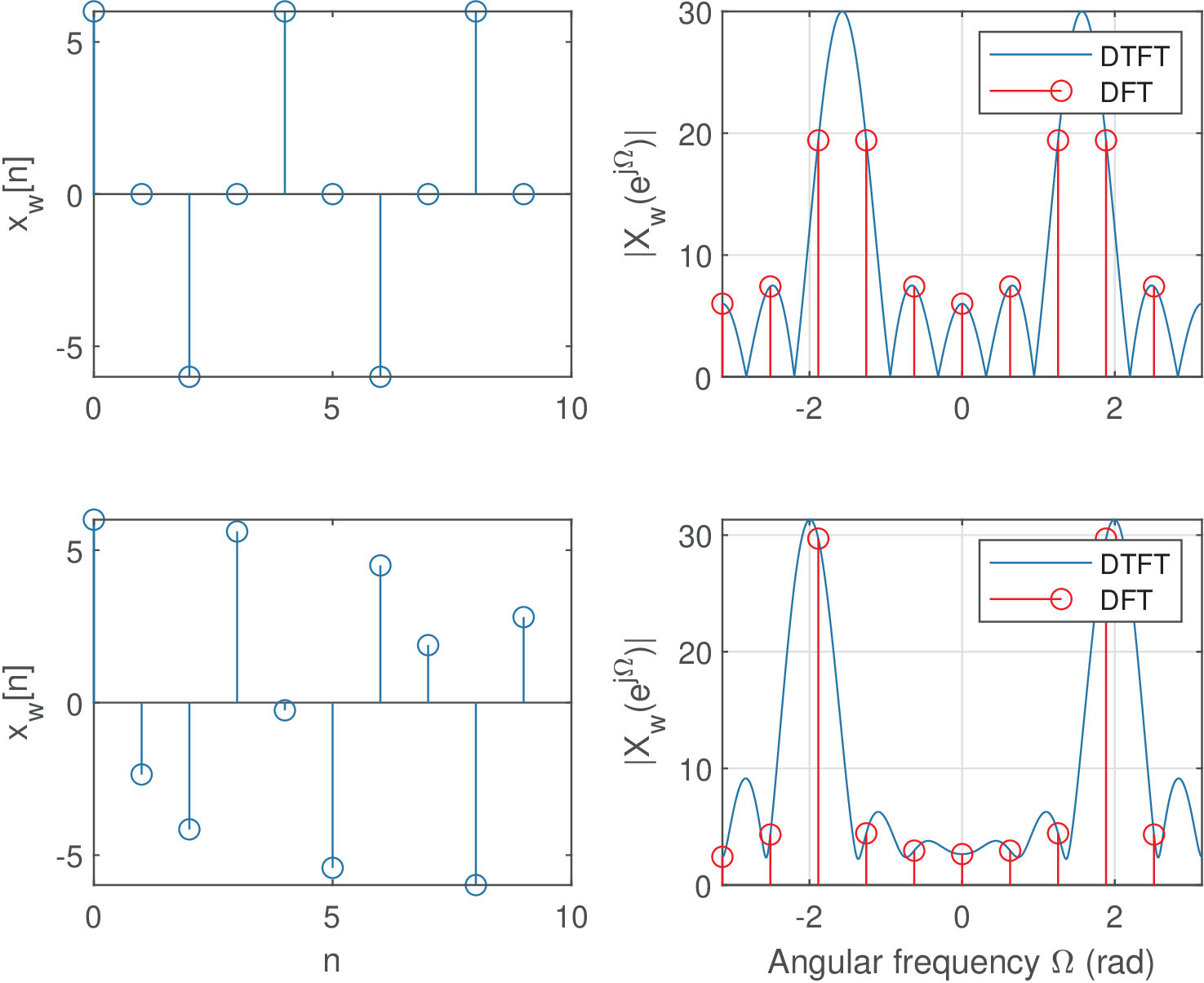
The bottom plots of Figure 4.19 were obtained from a non-periodic signal , but the DFT result presents a stronger peak than its top plot counterpart. By observing only the top DFT, one could be confused whether is composed of one or two sinusoids. On the other hand, observing the bottom DFT could lead to concluding that is periodic, while strictly it is not. The idea of Figure 4.19 is that care must be exercised when interpreting FFT results.
Another couple of examples is provided. Assume now that the signal of interest is , with and , where is the adopted length of the rectangular window and FFT size. In this special case, in which , the fundamental period is samples, given that simplifying the fraction leads to , and this cosine is represented by the FFT bins (note that the negative frequency would correspond to when fftshift is not used). The DTFT and FFT magnitudes of are depicted at the left plot in Figure 4.20.
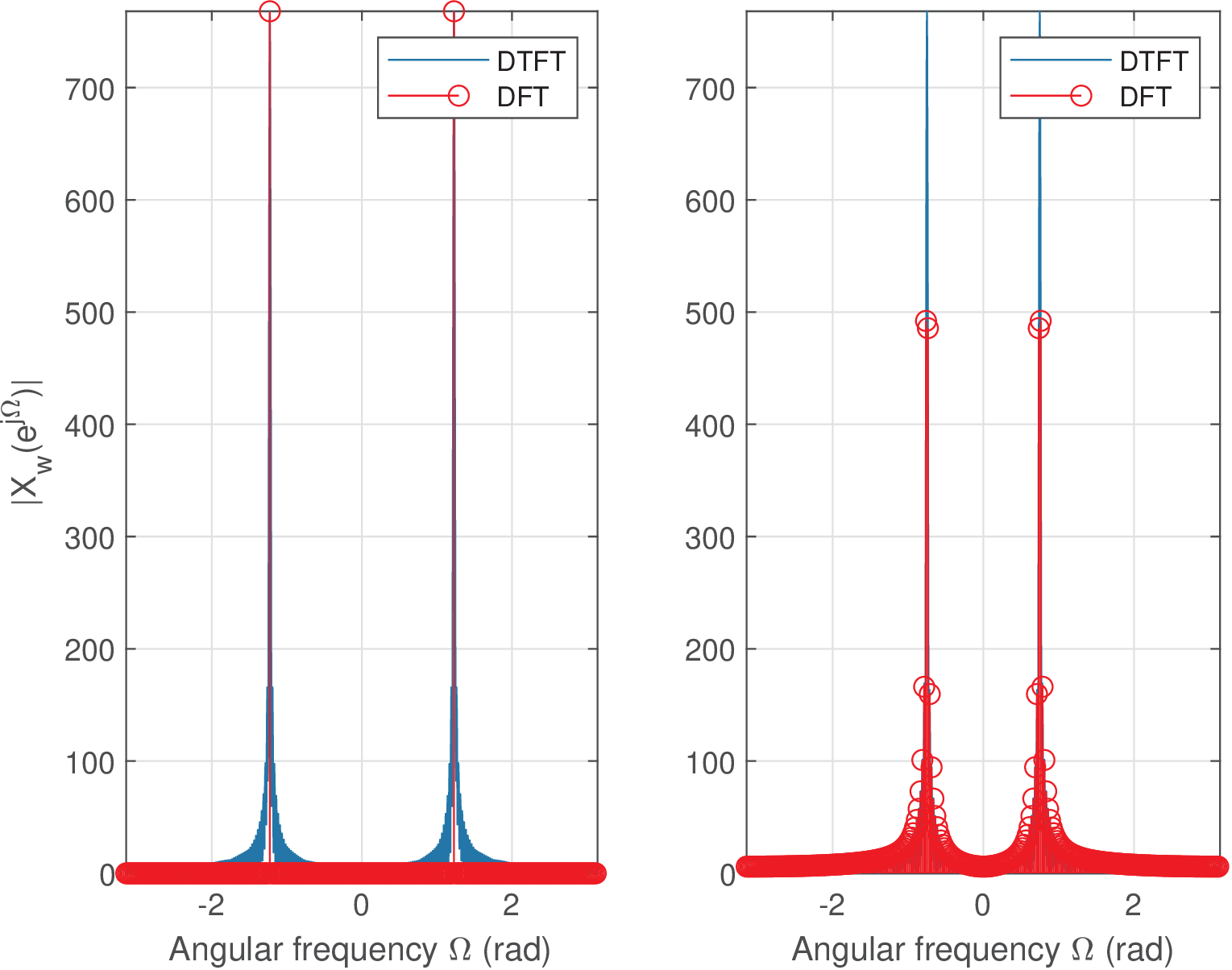
The right plot in Figure 4.20 used the signal , still with a window and FFT size . In this case, and , but and can be written as a ratio of two integers and . The signal has a period of samples but only of its samples are being analyzed via the FFT. In this case, the FFT does not “see” a pure sinusoid. The component of corresponding to the positive frequency will reside between the bins and , while the negative-frequency component will be located between bins and . Leakage will occur for both components and will be more visible in their neighbor bins.
4.3.6 Frequency resolution of the overall spectral analysis
In previous paragraphs, we observed that reduced resolution and leakage are the two primary effects on the spectrum as a result of applying a window to the signal. The resolution of the overall spectral analysis is primarily influenced by the width of the main lobe of the window, which is inversely proportional to the window (and consequently signal) duration. The degree of leakage depends on aspects of the window DTFT such as the relative amplitude of the main lobe with respect to the amplitudes of the sidelobes.
An FFT-based spectral analysis resolution also depends on the FFT resolution as described by Eq. (2.37), with being the number of FFT points. Given a windowed signal with duration of samples, the FFT resolution can always be improved via zero-padding and adopting .
In summary, there are two artifacts to be consider when calculating the resolution of a FFT-based spectral analysis:
- Leakage, which becomes stronger when the window duration is made shorter (or equivalently, made smaller)
- FFT resolution , which can be improved by increasing the number of FFT points and using zero-padding.
These two effects appear in a combined way in FFT-based spectral analysis. And while improves as gets larger, this cannot recover the leakage that occurred due to windowing.
These effects appear in a combined way in FFT-based spectral analysis, such as in Application 2.10.
4.3.7 Example of using windows in spectral analysis
To illustrate the importance of windows other than the rectangular, two distinct signals, and , each composed by a stronger and a weaker sinusoids, will have their spectra estimated using a FFT with points:
-
Case 1: the stronger sinusoid is bin-centered - The first sequence is
The idea is that the weaker cosine (of amplitude 1 V) is located in the center of the FFT bin , and the stronger is located in the center of bin 38. Having a bin-centered sinusoid corresponds to choosing the FFT size coinciding with a multiple of the sinusoid period.
-
Case 2: the stronger sinusoid is not bin-centered - The second sequence is
In this case, the weaker cosine is located in the center of bin 32 but the stronger is located in the border of bins 37 and 38.
In this example the goal is to distinguish the sinusoids and estimate their frequencies. As in many applications of spectral analysis, the amplitudes are irrelevant and what is taken into account is the relative difference between the signal components in frequency domain. For both and , the difference in power between the sinusoids is dB. These sequences can be generated as in Listing 4.4.
1N=256; %number of samples available of x1 and x2
2n=0:N-1; %abscissa
3kweak=32; %FFT bin where the weak cosine is located
4kstrong1=38; %FFT bin for strong cosine in x1
5weakSigal = 1*cos((2*pi*kweak/N)*n+pi/3); %common parcel
6x1=100*cos((2*pi*kstrong1/N)*n+pi/4) + weakSigal; %x1[n]
7kstrong2=37.5; %location for strong cosine in x2
8x2=100*cos((2*pi*kstrong2/N)*n+pi/4) + weakSigal; %x2[n]
The commands that design the windows to pre-multiply x1 and x2 in Listing 4.4, before calling the FFT, are given in Listing 4.1.
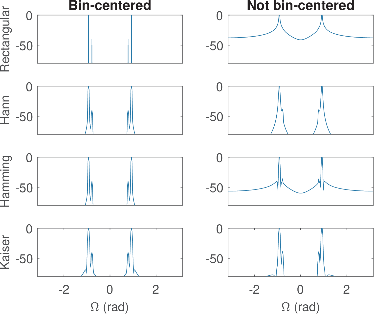
The results with four windows from Listing 4.1 are shown in Figure 4.21. The flat top window was not used due to its poor frequency resolution. For example, the spectrum in Figure 4.21 for (called x2 in the code) using Hamming was obtained with Listing 4.5.
1N=256; n=0:N-1; %N is the number of available samples and FFT length
2x2=100*cos((2*pi*37.5/N)*n+pi/4) + cos((2*pi*32/N)*n+pi/3); %cosines
3dw=(2*pi)/N; %DFT spacing in radians
4w=-pi:dw:pi-dw; %abscissa for plots matched to fftshift
5x=x2.*hamming(N)'; %perform windowing
6factor=max(abs(fft(x))); %normalization to have stronger at 0 dB
7plot(w,fftshift(20*log10(abs(fft(x)/factor))));
The graphs at the left column in Figure 4.21 correspond to estimated spectra of (both sinusoids are bin-centered). For , it can be seen that the best result was obtained by a rectangular window while the other windows led to spectra with leakage (spurious power) near the cosines. Based solely on the results obtained for case 1, one could erroneously concluded that the rectangular window is always the best. However, as shown in the top-right graph, when the strong cosine is not bin-centered, the rectangular window miserably fails to detect the weaker cosine.
In Figure 4.21, the Hann window allows a marginal detection of the weaker cosine, while the Hamming window allows the detection of both cosines but contaminates the whole spectrum with spurious power along frequency just 50 dB below the power level of the strongest sinusoid. This is a consequence of the reduced side-lobe fall-off for the Hamming window, as indicated in Figure 4.3. The Kaiser window achieves the best result when one takes in account both cases (bin-centered and not).
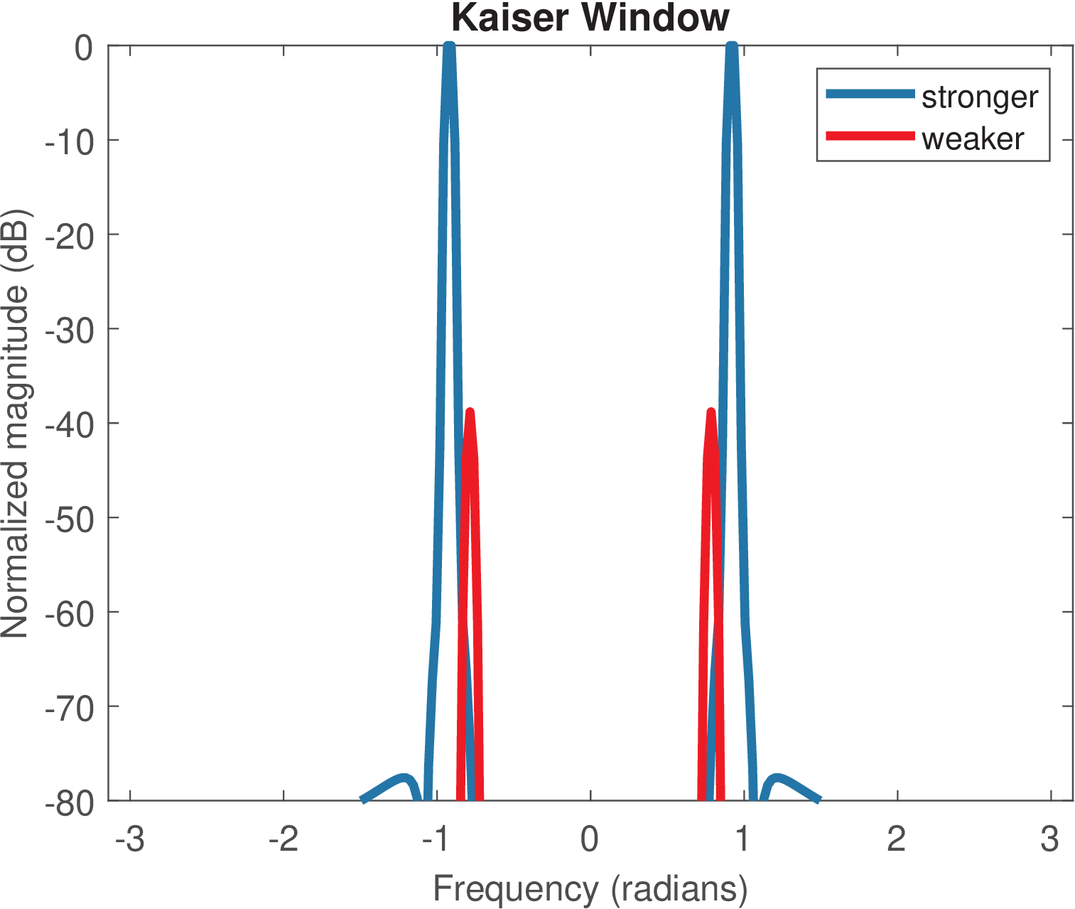

To complement the analysis of estimating the spectrum of (the stronger sinusoid is not bin centered), Figure 4.22 and Figure 4.23 show the individual spectra of the two sinusoids superimposed, obtained using the Kaiser and rectangular windows, respectively. Note that, Figure 4.21 shows exactly the combined effect of these individual spectra. Figure 4.23 clearly shows that the significant leakage of the stronger cosine caused by the rectangular window, completely “masks” the weaker cosine.
Note that this was a specific application. For example, features such as side-lobe fall-off are important in other situations. A very general conclusion is to always use a window other than the rectangular when performing spectral analysis of a signal that is not guaranteed to have all components bin-centered. And, if possible, adopt different windows to benefit from their best features to interpret the signal under analysis.
To conclude the discussion on windowing, the following example explores how to properly apply the theory in practice, when dealing with DTFTs that contain impulses.
Example 4.4. Advanced: When a DTFT has impulses, does this create a problem for an FFT-based analysis?. A DTFT can have impulses such as, for example, the DTFT of a sinusoid. One question that may arise then is: -If the FFT simply performs sampling of the DTFT in the frequency domain, what is the FFT value when exactly sampling an impulse? Should this value go to infinite? The answer requires noting that the impulse in the DTFT appears because is an infinite-long signal (e. g., an infinite-length sinusoid). But an FFT has to be applied to a signal with a finite number of samples. Therefore, the FFT is always applied to a windowed signal , with a DTFT that does not have impulses.
After this introduction to windowing, the next sections discuss three important functions in spectral analysis: ESD, PSD and MS Spectrum. While the PSD targets power signals, the ESD is a convenient tool for analyzing energy signals, informing how the total energy is distributed over frequency. Both are “density” functions, with the independent variable . The mean-square (MS) spectrum is a discrete-frequency function with the independent variable . We will discuss each of the three functions in the next sections.