Nonparametric PSD Estimation via Periodogram

4.6 Nonparametric PSD Estimation via Periodogram

The ESD, PSD and MS spectrum were defined without a discussion on how to estimate them. This section will exclusively concern the estimation of PSDs using the FFT, as indicated in Figure 4.26. The PSD estimation methods can also be used to estimate the ESD and MS spectrum.

Figure 4.26: ESD, PSD and MS spectrum with respective units, and two methods for estimating PSDs that can also be used to estimate the ESD and MS spectrum.

The periodogram $Ŝ [k]$ is a classical approach for PSD estimation. There are distinct definitions in the literature and here, especially for consistency with Matlab/Octave, the periodogram is an approximation of $S (f)$ and defined as

Ŝ [k] \overset{def}{=} \frac{1}{N BW} | FFT {x_{N} [n]} |^{2},

(4.47)

where $x_{N} [n]$ is the $N$ -samples windowed version of $x [n]$ and $BW$ the assumed frequency bandwidth. If the window is other than the rectangular, $Ŝ [k]$ is called the modified periodogram.

When compared to the actual PSD $S (f)$ , notice that the periodogram $Ŝ [k]$ may present aliasing in case $x_{N} [n]$ was obtained by sampling a continuous-time $x (t)$ . It may also present leakage due to windowing. Besides, the periodogram inherits the properties and pitfalls of an FFT, such as a frequency resolution $Δ Ω = 2 π ∕ N$ that may not be enough to distinguish peaks separated by less than $Δ Ω$ due to the picket-fence effect.

Based on the definition of $Ŝ [k]$ , the signal power $P$ can be conveniently obtained by approximating the integral of Eq. (4.19). For instance, using the rectangle method one obtains

P \approx Δ f \sum_{k = 0}^{N - 1} Ŝ [k],

(4.48)

where $Δ f = BW ∕ N$ is the FFT frequency spacing.

Some important facts related to this definition:

The periodogram is associated by definition to the FFT operation and, consequently, operates on a finite-length discrete-time signal.
The periodogram input is a discrete-time signal, but frequencies can be conveniently interpreted in Hertz (or rad/s) via $ω = F_{s} Ω$ (Eq. (1.36)) when the sampling frequency $F_{s}$ is specified.
The analysis bandwidth $BW$ is in Hertz, and obtained from the specified sampling frequency $F_{s}$ . The $BW$ is assumed to be from $- F_{s} ∕ 2$ to $F_{s} ∕ 2$ for a bilateral or $0$ to $F_{s} ∕ 2$ for a unilateral periodogram.

Matlab/Octave adopted conventions for periodograms

Is should be noted that Matlab/Octave adopts the following:

When the sampling frequency $F_{s}$ is not specified, it is assumed $F_{s} = 2 π$ and Eq. (4.19) is adopted.
When $F_{s}$ is specified, the PSD frequency axis (abscissa) is assumed to be in Hertz. When $F_{s}$ is not specified the frequency axis unit is assumed to be “rad/sample” (which corresponds to $Ω$ in radians according to the nomenclature adopted in this text).
When the signal is real, a unilateral PSD is adopted by default.
By default, the periodogram.m function uses a power-of-two FFT-length with a minimum of 256, adopting zero-padding in case the input signal has less than 256 samples.
The periodogram values are converted to dB scale.

These conventions are discussed in the sequel.

As mentioned, a characteristic of Matlab/Octave is the adoption, by default, of a unilateral PSD when the signal is real and has a Hermitian-symmetric spectrum. In this case, only the nonnegative frequency range are used in the graphs and in the summation of the normalized periodogram to obtain $P$ . For example, in continuous-time, instead of Eq. (4.48), one would have

P = \int_{0}^{\infty} S (f) d f \approx Δ f ∑_{k = 0}^{(N ∕ 2) + 1} Ŝ [k],

(4.49)

assuming $N$ is even. Hence, the values of $Ŝ [k]$ in a unilateral periodogram are twice the values in the corresponding bilateral representation, with exception of the DC and Nyquist frequencies.

4.6.1 Periodogram of periodic signals and energy signals

A periodogram must be properly interpreted if applied to a periodic signal. Note that, as indicated in Section 4.4.3.0, while the PSD of a periodic signal is composed by impulses, the periodogram $Ŝ [k]$ obtained from a finite-duration window does not contain impulses due to the convolution between the original spectrum and the window spectrum. This issue was discussed in Section 4.3.7.0. Besides, a periodogram indicates the power distributed in bins with width $Δ f$ Hz. Hence, if a sinusoid of power $P$ is located at a bin center, the periodogram estimates the corresponding PSD level as $P ∕ Δ f$ This is a fact that needs always to be taken in account when using a periodogram to represent a periodic signal that has impulses in its continuous-time PSD $S (f)$ .

Care must also be exercised when a periodogram is applied to an energy signal. As discussed in Section 4.4.1, an energy signal should be associated to an ESD, not PSD. The periodogram of an energy signal such as $x [n] = u [n] - u [n - 5]$ , for example, is implicitly assuming that $x [n]$ is just a windowed version of a periodic signal.

4.6.2 Examples of continuous-time PSD estimation using periodograms

Before discussing more advanced concepts such as the Welch method for PSD estimation, few examples of periodograms are provided in this section to consolidate the basic theory.

Example 4.11. Using periodogram.m to approximate the continuous-time PSD $S (f)$ of a sinusoid. When the sampling frequency $F_{s}$ is specified as input argument and without output arguments, the periodogram of Matlab/Octave indicates the abscissa in Hertz. For example, Listing 4.7 was used to generate Figure 4.27, which has the abscissa going from 0 to $F_{s} ∕ 2$ Hz because the signal is real and the default periodogram is unilateral in this case.

Listing 4.7: MatlabOctaveCodeSnippets/snip_frequency_normalized_periodogram.m. [ Python version]

1N=1024; A=10; x=A*cos(2*pi/64*(0:N-1));%generate cosine 
2Fs=8000; %sampling frequency in Hz 
3rectWindow=rectwin(N); %rectangular window 
4rectWindow=rectWindow(:); x=x(:); %make sure both are column vectors 
5[P,f]=periodogram(x,rectWindow,N,Fs); %periodogram 
6df = Fs/N; %FFT bin width to be used in power computation 
7Power=sum(P)*df %calculate the average power 
8plot(f/1000,10*log10(P)); grid, %convert to dBW/Hz

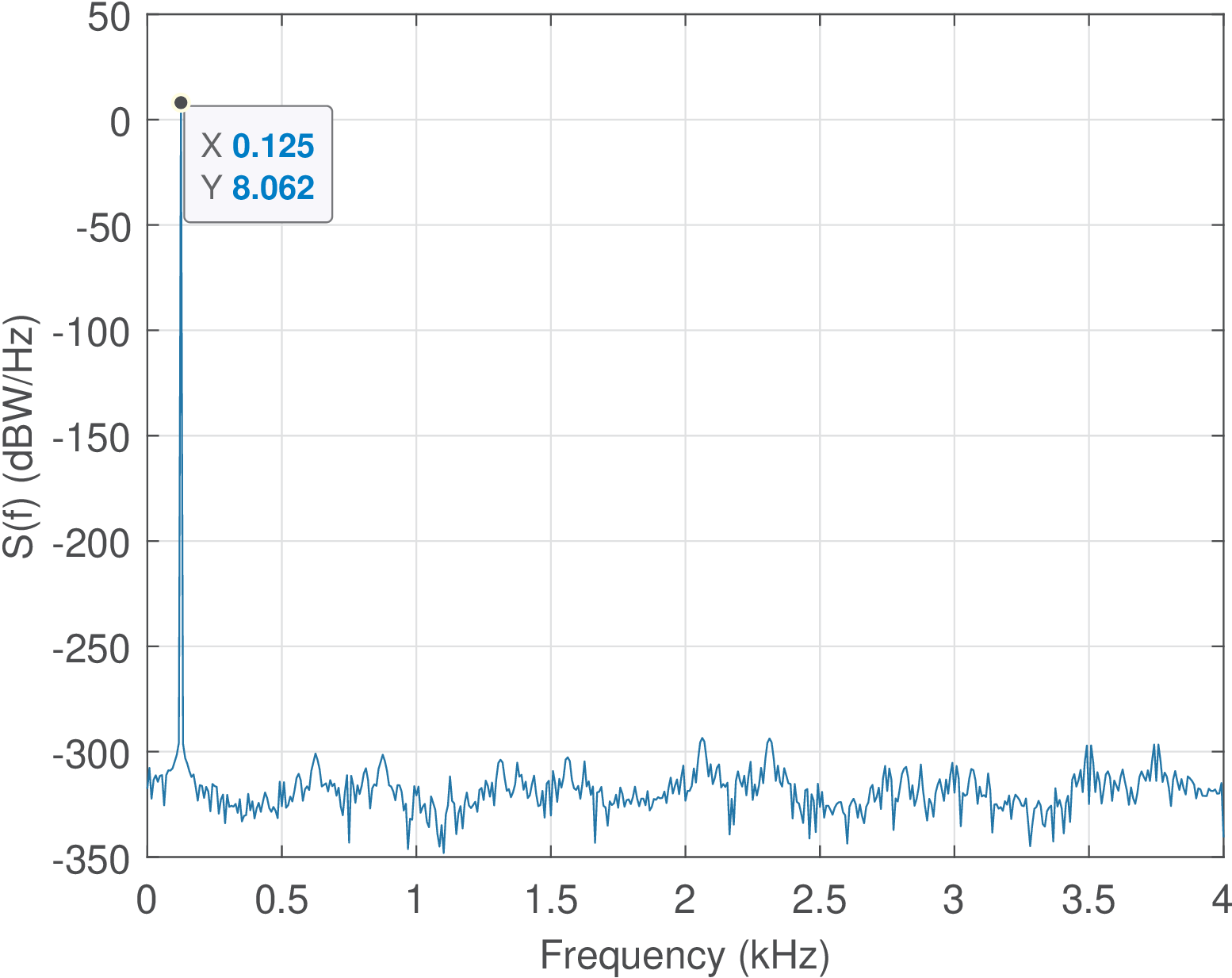
Figure 4.27: Periodogram of $x [n] = 10 cos ((2 π ∕ 64) n)$ in dBW/Hz estimated by periodogram.m with a $1024$ -point FFT and assuming $F_{s} = 8$ kHz.

The signal power is $P = 50$ W. Figure 4.27 indicates a peak at $f = 125$ Hz, which corresponds to tone $k = 16$ . This can be confirmed by observing that $Δ f = F_{s} ∕ N = 8000 ∕ 1024 \approx 7.8125$ Hz, such that $f_{k} = k Δ f = 16 \times 8000 ∕ 1024 = 125$ Hz. Because there was no visible leakage in this case, the sinusoid power $P = 50$ W is completely residing in bin $k = 16$ . When using periodograms to represent sinusoids, as explained in Section 4.6.1, the sinusoid power is divided by the frequency range of the bin (the bin width). Hence, from Eq. (4.51), the expected PSD value at this bin is $Ŝ [k] |_{k = 16} = P ∕ Δ f = 50 ∕ 7.8125 = 6.4$ W/Hz. Converting it to dBW leads to $10 {log}_{10} 6.4 \approx 8.062$ dBW/Hz, as indicated in Figure 4.27. In summary, the PSD value in W/Hz at a given FFT bin is the power in watts concentrated in this bin divided by the bin width in Hz.

One aspect of PSD graphs in dB scale is that dynamic ranges larger than hundreds of dB should be associated to numerical errors, given that 10*log10(eps)=-156.5. $□$

Example 4.12. The power ratio between sinusoids can be obtained via PSDs.

Listing 4.8 provides an example of a signal composed of the sum of two bin-centered sinusoids. The periodogram is calculated via Matlab/Octave and also according to its definition (Sdef). Both ways lead to the same results, because the periodogram used the default rectangular window. Adopting a different window would lead to discrepant results. The power calculated in time (Power_time) and frequency (Power_freq) domains also coincide, having the value of 50.5 W. Figure 4.28 shows the graph generated by Listing 4.8.

Listing 4.8: MatlabOctaveCodeSnippets/snip_frequency_cosines_psd.m. [ Python version]

1N=128; n=(0:N-1)'; %number of samples and column vector 
2Fs=2000; %bandwidth in Hertz, equivalent to sampling frequency 
3dW=(2*pi)/N; %FFT bin width in radians, to define cosines 
4k1=N/4; k2=N/8; W1=k1*dW; W2=k2*dW;%define frequencies in radians 
5x=10*cos(W1*n) + 1*cos(W2*n); %create sum of bin-centered cosines 
6Sdef = (abs(fft(x)).^2)/(N*Fs); %periodogram via its definition 
7Sdef = [Sdef(1); 2*Sdef(2:N/2); Sdef(N/2+1)]; %convert to unilateral 
8[S,f] = periodogram(x,rectwin(N),N,Fs); %using periodogram function 
9Power_freq=(Fs/N)*sum(S) %estimate power (watts) in frequency domain 
10Power_time=mean(x.^2) %estimate power (watts) in time domain 
11h=plot(f,10*log10(Sdef),'-x'); hold on 
12h2=plot(f,10*log10(S),'-ro'); %Periodogram (dB scale) 
13legend('via definition','via Matlab') 
14xlabel('f (Hz)'), ylabel('S(f) (dBW/Hz)') 
15%use w=W Fs to convert to f in Hz and show datatips (f=W*Fs/(2*pi)) 
16f1=W1*Fs/(2*pi); f2=W2*Fs/(2*pi); %frequencies in Hz 
17datatip(h,f1,Sdef(k1)); datatip(h,f2,Sdef(k2));

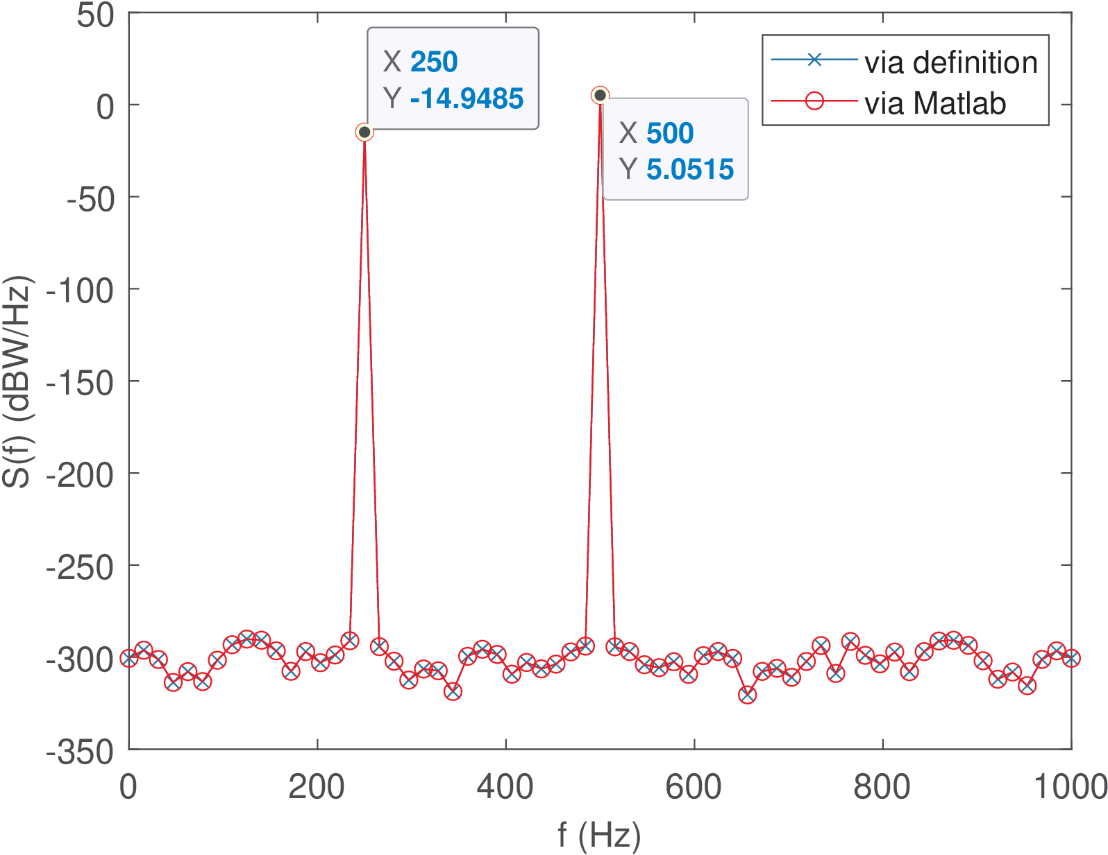
Figure 4.28: Periodogram of two bin-centered sinusoids at 250 and 500 Hz, calculated via Matlab and its definition.

The amplitudes of the sinusoids are 10 and 1 V, corresponding to power values of $P_{1} = 50$ and $P_{2} = 0.5$ W, respectively. These values in dB scale correspond to 16.9897 and $- 3.0103$ dBW, which corresponds to a power ratio $P_{1} ∕ P_{2} = 50 ∕ 0.5 = 100$ in dB of $16.9897 - (- 3.0103) = 10 {log}_{10} (P_{1} ∕ P_{2}) = 20$ dB.

Given that the bin width is $F_{s} ∕ N = 2000 ∕ 128 = 15.625$ Hz, the PSD values are $50 ∕ 15.623 \approx 3.2$ and $0.5 ∕ 15.623 \approx 0.032$ at their corresponding frequencies of 500 and 250 Hz, respectively. The PSD values in dBW/Hz are $10 {log}_{10} 3.2 \approx 5.0515$ and $10 {log}_{10} 3.2 \approx - 14.9485$ dBW/Hz. Note that subtracting the PSD values leads to $5.0515 - (- 14.9485) = 20$ dB, as obtained when manipulating the power values. This is an interesting aspect: the relative difference in power between the two sinusoids can be directly obtained from the periodogram (or equivalently, from the PSD). The estimated PSD graph does not allow directly reading the absolute power values but explicitly informs the relation between powers of signal components that reside in single bins.

We now modify the call to the periodogram function to use the Hamming window with [S,f] = periodogram(x,hamming(N),N,Fs) in Listing 4.8. The corresponding result is depicted in Figure 4.29, which compares the periodograms with rectangular and Hamming windows. As mentioned in Section 4.6, the latter is called a “modified” periodogram.

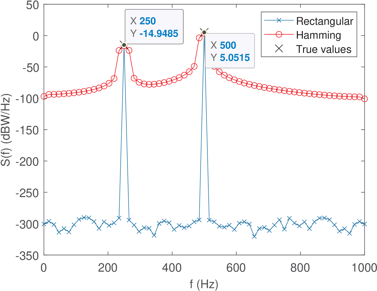
Figure 4.29: Periodograms of two bin-centered sinusoids at 250 and 500 Hz, calculated with the rectangular and Hamming windows.

Figure 4.29 shows a clear advantage of the rectangular window in this case in which the two sinusoids are bin-centered. We modify again the script in Listing 4.8 to position the cosine frequencies halfway of bin centers with k1=N/4+0.5; k2=N/8+0.5. This leads to the frequencies f1=507.8125 and f2=257.8125 Hz. Figure 4.30 shows the corresponding results.

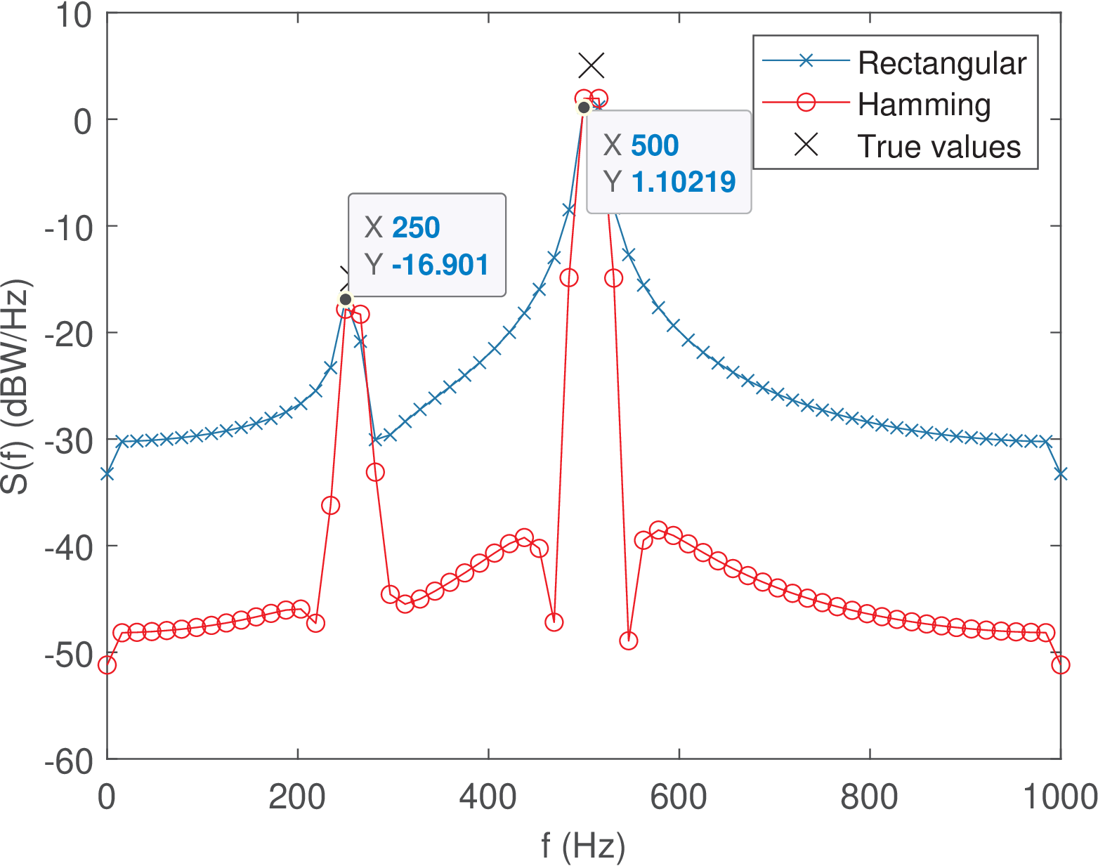
Figure 4.30: Periodograms of two non-bin-centered sinusoids at f1=507.8125 and f2=257.8125 Hz calculated with the rectangular and Hamming windows.

Figure 4.30 shows datatips for the rectangular-window periodogram at the FFT bin centers corresponding to 250 and 500 Hz, which are the bins in the FFT frequency grid immediately before the cosine frequencies f1=507.8125 and f2=257.8125 Hz. In this case, both rectangular and Hamming periodograms do not achieve the correct (“true”) PSD values neither in frequency nor in amplitude. For instance, the periodogram with the rectangular window indicates a PSD value of 1.10219 dBW/Hz at 500 Hz for the stronger cosine, while the true value is 5.0515 dBW/Hz at 507.8125 Hz, as indicated in Figure 4.28. $□$

Example 4.13. PSD of a sinusoid contaminated by AWGN. Special care must be exercised when interpreting a PSD that represents both broadband and narrowband signals. An example is when using the PSD to estimate the SNRs of sinusoids immersed in white noise. Figure 4.31 shows the periodogram of a cosine contaminated by AWGN generated with Listing 4.9.

Listing 4.9: MatlabOctaveCodeSnippets/snip_frequency_noisy_cosine.m. [ Python version]

1N=1024; A=4; %# of samples and cosine amplitude of A Volts 
2Fs=8000; Ts=1/Fs; %sampling frequency (Hz) and period (s) 
3f0=915; %cosine frequency in Hz 
4noisePower=16; %noise power in Watts 
5noise=sqrt(noisePower)*randn(1,N); 
6t=0:Ts:(N-1)*Ts; %N time instants separated by Ts 
7x=A*cos(2*pi*f0*t) + noise;%generate cosine with AWGN 
8[P,f]=periodogram(x,[],N,Fs); %periodogram (using the default window) 
9plot(f,10*log10(P)); %plot in dB scale

Listing 4.9 was used to generate the top plot with subplot(211). Then, the bottom plot was obtained by increasing N from 1024 to 16384. All the absolute values of the two periodograms differ due to their dependence on N.

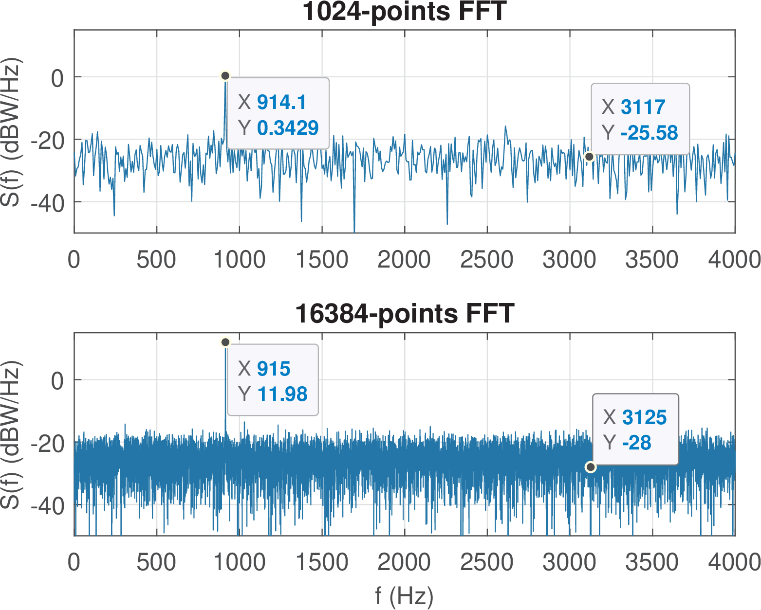
Figure 4.31: Periodograms of a cosine contaminated by AWGN at an SNR of $- 3$ dB with an FFT of $N = 1024$ points (top plot) and 16384 (bottom). In this case the SNR cannot be inferred directly from the noise level.

It can be noticed from Listing 4.9 that the cosine power is $P_{c} = A^{2} ∕ 2 = 8$ W while the noise power is 16 W, leading to a $SNR = 10 {log}_{10} (8 ∕ 16) \approx - 3.01$ dB. However, one may be tempted by Figure 4.31 to erroneously infer that SNR is positive given that the noise level (sometimes called noise floor) is more than 20 dB below the cosine peak for the top graph. Directly observing the ratio of powers in PSD graphs was valid in Figure 4.33, but in that case, the cosines were assumed to have all power confined in their respective bins. This is not the case with signals that have power spread over several bins and especially with white noise.

Because the white noise power is spread over all bins of a periodogram, the larger the number $N$ of FFT bins, the less noise power each bin carries and the larger the difference between the sinusoid power (assumed to be confined in a single bin) and the noise floor. In Figure 4.33, the bottom plot shows that the cosine power is approximately 30 dB above the noise level when N is increased to 16384. However, in both plots, the SNR is $- 3$ dB as attested by Listing 4.9.

In summary, the proper way of measuring the signal power is to account for the power in all bins that represent the signal. $□$

Example 4.14. Bilateral versus unilateral periodograms. The bilateral and unilateral periodograms are contrasted in Listing 4.10 and Listing 4.11.

Listing 4.10: MatlabOctaveCodeSnippets/snip_frequency_comparePeriodograms.m. [ Python version]

1N=1024; n=(0:N-1)'; %number N of samples and column vector n 
2A=10; x=A*cos((2*pi/64)*n); %generate cosine with period 64 
3BW = 2*pi; %assume defaut Fs=2*pi (bandwidth) in periodogram 
4S = abs(fft(x)).^2/(BW*N); %Periodogram (|FFT{x}|^2)/(BW * N) 
5Nfft = N; %force the FFT size in the periodogram below: 
6[Suni,w]=periodogram(x,[],Nfft); %Unilateral periodogram 
7Power = sum(Suni)*BW/N %Power from unilateral periodogram 
8Power2 = sum(S)*BW/N %Power from bilateral periodogram 
9Sunilateral2 = [S(1); 2*S(2:N/2); S(N/2+1)]; %from bi to unilateral 
10plot(w,Suni,'-o',w,Sunilateral2 ,'-x') %Compare periodograms

As indicated in Listing 4.10, to obtain the power $P$ from the periodogram, the proper normalization factor is the bin width $Δ f$ =BW/N for both cases, uni and bilateral. In this case $Δ f = 2 π ∕ 1024$ because $F_{s}$ was not specified when calling the periodogram.m routine and the default $F_{s} = 2 π$ is assumed.

A minor detail is that when $N$ is even and the periodogram is unilateral, f_uni(end) is $F_{s} ∕ 2$ Hz and length(f_uni) is $(N ∕ 2) + 1$ . Listing 4.11 illustrates this point by indicating in the last line of the script that length(f_uni) $= 513$ samples and f_uni(end) $= 250$ Hz, given that $N = 1024$ in this case.

If a bilateral periodogram is calculated, f_bil(end) is $(F_{s} ∕ 2) - Δ f$ and length(f_bil) is $N$ . The script in Listing 4.11 indicates that length(f_bil) $= 1024$ samples and f_uni(end) $= 499.5117 = 500 - Δ f$ Hz.

Listing 4.11: MatlabOctaveCodeSnippets/snip_frequency_correctPeriodograms.m. [ Python version]

1N=1024; n=(0:N-1)'; %number N of samples and column vector n 
2A=10; x=A*cos((2*pi/64)*n); %generate cosine with period 64 
3Fs=500; BW = Fs; %Fs = BW = 500 Hz 
4[S_uni,f_uni] = periodogram(x,[],N,Fs); %Unilateral periodogram 
5[S_bil,f_bil] = periodogram(x,[],N,Fs,'twosided'); %Bilateral period. 
6Power = (BW/N)*sum(S_uni) %Power for unilateral periodograma 
7Power2 = (BW/N)*sum(S_bil) %Power for bilateral periodograma 
8length(f_uni),f_uni(end),length(f_bil),f_bil(end) %values for N even

All the previous calculations in Listing 4.10 and Listing 4.11 (e. g., sum(S)) used the periodogram in linear scale. But another convention adopted by Matlab/Octave is to convert, by default, the periodogram values to dBW/Hz when the function periodogram.m is invoked without output parameters. As we warned in Appendix A.24, the periodogram unit is informed to be dB/Hz instead of dBW/Hz. We consider the latter option more appropriate to emphasize that is an absolute value of power density instead of a relative (dB) value. $□$

4.6.3 Relation between MS spectrum and periodogram

The FFT-based estimations of PSD and MS spectrum are closely related. From Eq. (4.36) and Eq. (4.47), the MS spectrum $Ŝ_{ms} [k]$ can be obtained by multiplying the periodogram $Ŝ [k]$ (PSD estimation) by the FFT frequency resolution $Δ f$ :

Ŝ_{ms} [k] = \frac{BW}{N} Ŝ [k] = Δ fŜ [k] .

(4.50)

In other words, the periodogram $Ŝ [k]$ (PSD estimation) can be obtained by dividing $Ŝ_{ms} [k]$ by $Δ f$ .

Because $Ŝ [k]$ is a PSD estimate, the user of a PSD estimation routine that returns $Ŝ [k]$ just needs to know the bin width $Δ f$ to be able to obtain the average power $P$ from $Ŝ [k]$ , and/or individual values of $Ŝ_{ms} [k]$ . This reasoning is valid when $P$ should be calculated over the whole frequency range, or shorter frequency intervals, because the amount of power $P_{k}$ at a single FFT bin (the $k$ -th bin) in a periodogram $Ŝ [k]$ is

Ŝ_{ms} [k] = P_{k} = Δ fŜ [k] .

(4.51)

For discrete-time signals assuming $BW = 2 π$ or $BW = 1$ , $P_{k} = (BW ∕ N) Ŝ [k]$ . In both continuous and discrete-time cases, $P = \sum_{k = 0}^{N - 1} P_{k}$ .

Listing 4.12 illustrates how Eq. (4.50) can be used to obtain $Ŝ_{ms} [k]$ .

Listing 4.12: MatlabOctaveCodeSnippets/snip_frequency_mssFromPeriodogram.m. [ Python version]

1N=1024; n=(0:N-1)'; %number N of samples and column vector n 
2A=10; x=A*cos((2*pi/64)*n); %generate cosine with period 64 
3Sms = abs(fft(x)/N).^2; %MS spectrum 
4BW = 1; %assumed bandwidth is 2*pi 
5S = abs(fft(x)).^2/(BW*N); %Periodogram (|FFT{x}|^2)/(BW * N) 
6Sms2=BW*S/N; %Example of obtaining MS spectrum from periodogram 
7Power = sum(Sms) %Obtaining power from the MS spectrum 
8Power2 = sum(S)*BW/N %Obtaining power from the periodogram

While the MS spectrum is a discrete function with the property specified by Eq. (4.37), the periodogram values $Ŝ [k]$ ideally coincide with a continuous function of frequency: the PSD $S (f)$ or $S (e^{j Ω})$ . Consequently, having an array of values $Ŝ [k]$ , the property that should be obeyed depends on the integral Eq. (4.19) or Eq. (4.21), respectively, not a summation as in Eq. (4.37).

It is recommended to observe Table A.1 and associated discussion, which summarizes an interesting analogy between the use of FFTs and histograms that helps understanding the difference betweeen $Ŝ [k]$ and $Ŝ_{ms} [k]$ .

4.6.4 Estimation of discrete-time PSDs using the periodogram

The periodogram is an approximation of the continuous-time PSD $S (f)$ , but one can “trick” the software routine and obtain an estimate of $S (e^{j Ω})$ by imposing $F_{s} = BW = 1$ Hz. In this case, the numerical values of the periodogram $Ŝ [k]$ provide an estimate $Ŝ (e^{j Ω})$ of the discrete-time PSD $S (e^{j Ω})$ as follows:

Ŝ (e^{j Ω}) |_{Ω = k (2 π ∕ N)} = Ŝ [k] .

(4.52)

Having the periodogram calculated with $F_{s} = 1$ , allows to interpret $Ŝ [k] ∕ (2 π)$ in watts/rad, as indicated in Eq. (4.18).

However, when invoking a periodogram software routine for discrete-time signals without specifying $F_{s}$ , the assumed default value is $F_{s} = 2 π$ , not $F_{s} = 1$ . The values of $Ŝ [k]$ will differ in these two cases by $2 π$ . But, independent on $F_{s}$ , the signal average power can always be obtained with Eq. (4.48).

4.6.5 Examples of discrete-time PSD estimation

Example 4.15. Discrete-time PSD of a sinusoid using the periodogram function. Listing 4.13 uses the Matlab/Octave periodogram function to estimate the discrete-time PSD of a cosine and compares it with a periodogram directly calculated based on the definition adopted in this text. Figure 4.32 depicts the result.

Listing 4.13: MatlabOctaveCodeSnippets/snip_frequency_periodogram.m. [ Python version]

1N=16; alpha=2; A=10; n=0:N-1; 
2x=A*cos((2*pi*alpha/N)*n); %generate cosine 
3x=x(:); %Octave requires column vector 
4BW=1; %it is a discrete-time signal, then assume BW=1 Hz 
5Sk = (1/(N*BW))*abs(fft(x)).^2; %Periodogram as defined in textbook 
6Power = (BW/N)*sum(Sk) %Obtain power from periodogram 
7Smatlab=periodogram(x,[],N,BW,'twosided'); %angular frequency in rad 
8M=length(Smatlab); %periodogram used zero-padding and unilateral PSD 
9Power2= (BW/N)*sum(Smatlab) %Power from periodogram function 
10%W= (2*pi/N)*(-N/2:(N/2-1)); %discrete frequency axis in radians 
11W= (2*pi/N)*(0:N-1); %discrete frequency axis in radians 
12clf; subplot(211); h=stem(W,Smatlab); 
13hold on; stem(W,Sk,'xr') 
14Npad=512; %use zero-padding to increase number of points to 253 
15[Smatlab,W]=periodogram(x,[],Npad,BW,'twosided'); %angular freq. in rad 
16subplot(212); stem(2*pi*W,Smatlab) 
17xlabel('\Omega (rad)'); ylabel('S(e^{\Omega})  (W/dHz)'); 
18datatip(h,2*pi/N,((A^2/2)/2)/(BW/N)) 
19%second figure 
20subplot(212); 
21[Smatlab,f]=periodogram(x,[],[],BW,'twosided'); %zero-padding 
22h=stem(2*pi*f,Smatlab,'xr'); 
23xlabel('\Omega (rad)'); ylabel('S(e^{\Omega})  (W/dHz)'); 
24datatip(h,2*pi/8,((A^2/2)/2)/(BW/N)) 
25axis tight

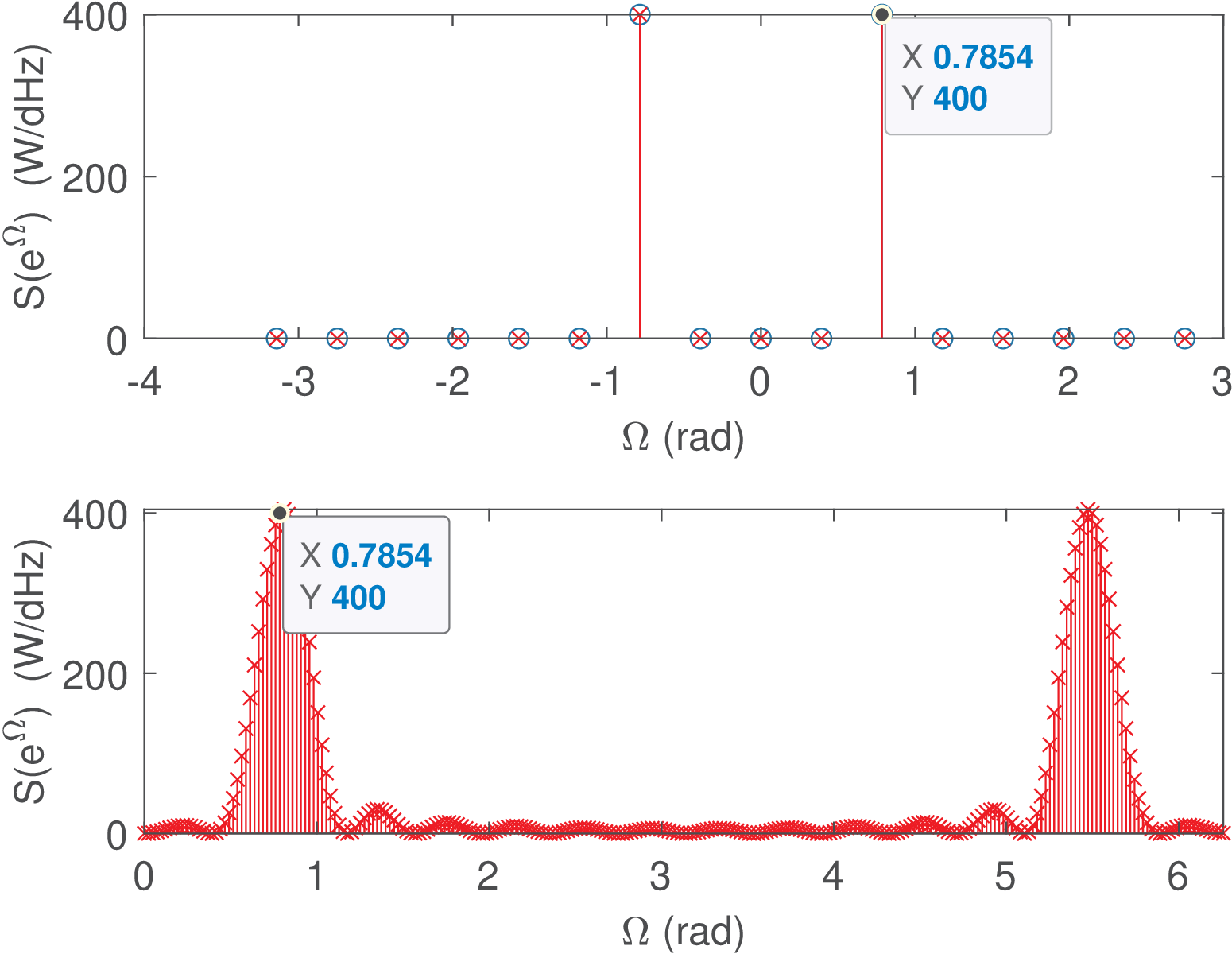
Figure 4.32: Discrete-time PSD of $x [n] = 10 cos ((2 π ∕ 8) n)$ in linear scale estimated with periodograms.

Listing 4.13 returns the value $P = 50$ W for both Power and Power2. The cosine angular frequencies are $\pm 0.7854$ rad as indicated in the top plot of Figure 4.32 for the positive frequency. The periodogram values at $k = - 2$ and $k = 2$ are $Ŝ [k] | k = \pm 2 = (P ∕ 2) ∕ Δ f = 400$ , given that $Δ f = BW ∕ N$ and $BW = 1$ .

There was no leakage in the top plot of Figure 4.32. But in case one allows the periodogram.m routine to use zero-padding as in:

1[Smatlab,f]=periodogram(x,[],[],BW,'twosided'); %zero-padding

the result is the bottom plot of Figure 4.32. In this case, periodogram.m adopted zero-padding to reach $N = 256$ samples. This can be confirmed with

1Power3= (BW/256)*sum(Smatlab) %Power from periodogram function

which returns Power3=50. Another discrepancy between the two plots in Figure 4.32 is that the bottom plot uses the range $Ω \in [0, 2 π [$ while the top plot adopted $[- π, π [$ via fftshift.m. $□$

Example 4.16. MS spectrum and PSD of a sum of discrete-time sinusoids. A 1024-points DFT is adopted to inspect a signal composed by two discrete-time cosines that are not bin-centered and have amplitudes 10 and 1 V, as indicated in Listing 4.14.

Listing 4.14: MatlabOctaveCodeSnippets/snip_frequency_not_bin_cent_cos.m. [ Python version]

1N=1024; n=(0:N-1)'; %number of samples and column vector 
2dw=2*pi/N; %FFT bin width 
3k1=115.3; k2=500.8; w1=k1*dw; w2=k2*dw;%define frequencies 
4x=10*cos(w1*n) + 1*cos(w2*n); %generate sum of two cosines 
5Sms = abs(fft(x)/N).^2; %MS spectrum |DTFS{x}|^2 
6[S,w] = periodogram(x); %Periodogram, frequency w=0 to pi 
7Power = sum(Sms) %estimate the power in Watts = A^2/2 
8k=0:N-1; %frequency index 
9subplot(211), h=plot(k,10*log10(Sms)); %MS spectrum (dB) 
10subplot(212), h2=plot(w,10*log10(S)); %Periodogram (dB)

Figure 4.33 depicts the obtained result. To obtain cosines that are not bin-centered, non-integer numbers k1=115.3 and k2=500.8 were specified to create the angular frequencies. Hence, each cosine has most of its power located at bins $k = 115$ and 501 as indicated by the data tips in Figure 4.33.

The top graph shows the bilateral MS spectrum with the positive frequencies (the ones that have associated data tips), from $k = 0$ to 512 preceding the “negative” frequencies from $k = 513$ to 1023. The function fftshift could be used to make the “negative” precede the positive frequencies. Note that the implicitly adopted rectangular window leads to considerable leakage. The bottom graph is a unilateral representation of the periodogram.

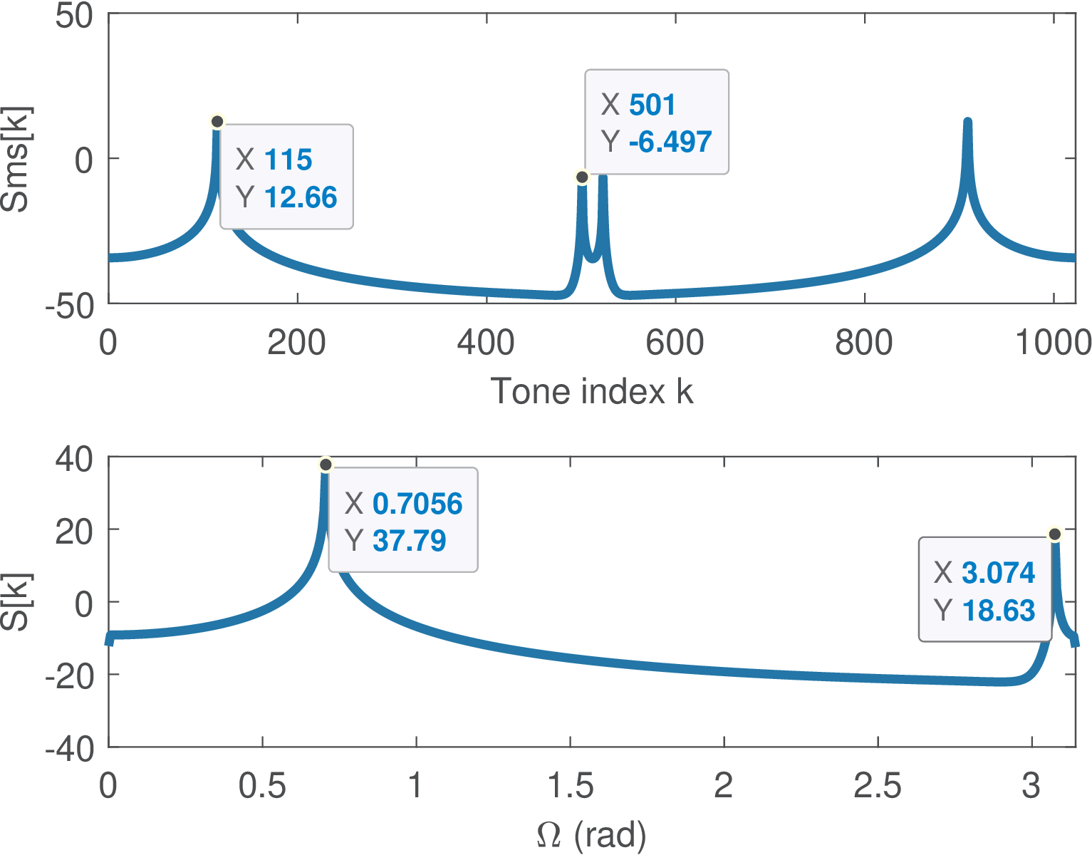
Figure 4.33: Periodogram and MS spectrum for a sum of sinusoids. Both are in dB scale.

The Power calculated by the code was 50.5397 W while the theoretical result for eternal sinusoids is $1 0^{2} ∕ 2 + 1^{2} ∕ 2 = 50.5$ . The small discrepancy is due to the fact that the sinusoids are not bin-centered and, consequently, the signal duration does not correspond to an integer number of periods of the sinusoids. Besides, one should notice that the time-domain signal x itself has power $P = 50.5397$ W, which coincides with Power.Bin-centered cosines with power 50 and 0.5 W would lead to values $10 {log}_{10} (25) \approx 13.98$ dB and $10 {log}_{10} (0.25) \approx - 6.02$ dB at their corresponding frequencies in a bilateral MS spectrum. Given that $BW = 2 π$ and the FFT bin width is $BW ∕ N = 2 π ∕ 1024 \approx 0.0061$ , the theoretical values for the unilateral periodogram are $10 {log}_{10} (50 ∕ 0.0061) \approx 39.11$ and $10 {log}_{10} (0.5 ∕ 0.0061) \approx 19.11$ . Figure 4.33 presents slightly smaller values for both MS spectrum and periodogram due to leakage. Because $BW = 2 π$ instead of $BW = 1$ , the depicted values are not the ones of a discrete-time PSD $S (e^{j Ω})$ .

An interesting aspect is that the relative difference in power between the two sinusoids can be obtained in both periodogram and MS spectrum, leading to $37.79 - 18.63 \approx 19.2$ dB and $12.66 - (- 6.497) \approx 19.2$ dB, respectively. In other words, the PSD does not allow directly reading the absolute power values but can inform the relation between powers of signal components that reside in specific bins. $□$

Example 4.17. Periodogram variance does not decrease with number of samples. Figure 4.34 illustrates the adoption of periodograms $Ŝ [k]$ to estimate the discrete-time PSD $S (e^{j Ω})$ of a white noise with power of 600 W. The estimation used $N = 300$ (top) and $N = 3000$ (bottom) samples of the noise signal. The code for signal generation and periodogram estimation for N=300 (the same code was used for N=3000 samples) is:

Listing 4.15: MatlabOctaveCodeSnippets/snip_frequency_noise_PSD.m. [ Python version]

1N = 300; % number of samples and FFT size 
2A=10; x=A*cos((2*pi/64)*n); %generate cosine with period 64 
3power_x = 600; %desired noise power in Watts 
4Fs = 1; %sampling frequency = BW = 1 
5x=sqrt(power_x) * randn(1,N); %Gaussian white noise 
6actualPower = mean(x.^2) %the actual obtained power 
7[Sk,F]=periodogram(x,[],[],Fs,'twosided'); %periodogram 
8subplot(211), plot(2*pi*F,Sk); %plot periodogram 
9Sx_th=power_x*ones(1,length(F)); %theoretical PSD 
10mean(Sk) %in this case, it coincides with actualPower 
11disp(['Periodogram standard deviation=' num2str(std(Sk))]) 
12hold on; h=plot(2*pi*F,Sx_th,'r:','lineWidth',3);

Note that due to the limited number N of samples, the actualPower values (e. g., 512.3 and 601.0 W), may differ from the desired value power_x=600.

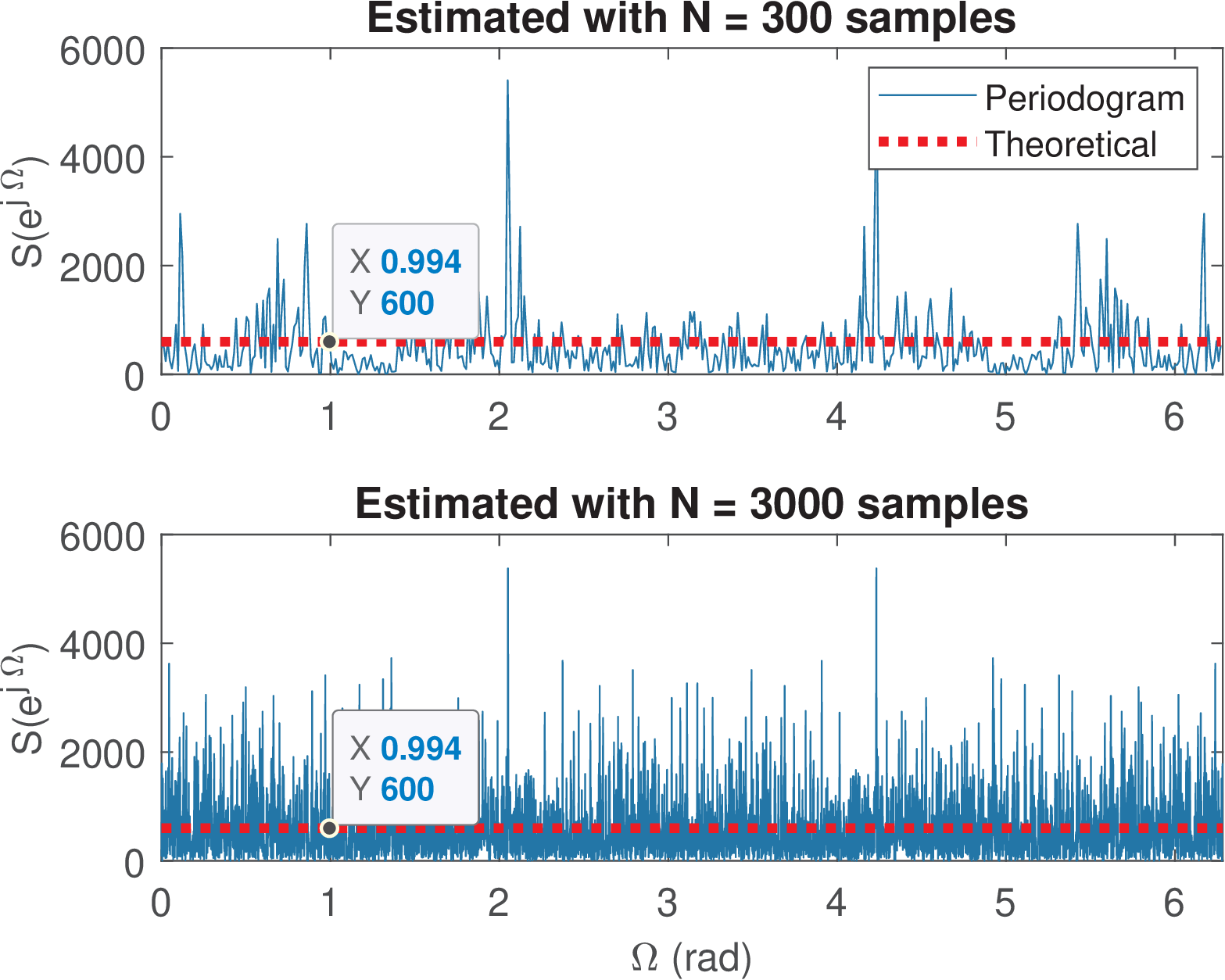
Figure 4.34: Periodograms of a white noise with power equal to 600 W estimated with $N = 300$ (top) and $N = 3000$ (bottom) samples.

Recall from Eq. (4.52), that in the case of $F_{s} = 1$ , the periodogram coincides with the discrete-time PSD estimate $Ŝ (e^{j Ω}) |_{Ω = k (2 π ∕ N)}$ .

This example illustrates that the periodogram values with $F_{s} = 1$ have an average mean(Sk) that coincides with actualPower (because $Δ f = 1 ∕ N$ in this case). However, the variance of the estimate does not decrease with $N$ . For $N = 300$ and 3000, the standard deviations are 593.1 and 599.4, respectively. This issue is discussed in Section 4.7, in which the Welch’s PSD estimation method is presented. $□$

4.6.6 Estimating the PSD from Autocorrelation

An alternative way of estimating the PSD of a finite duration discrete-time signal is via the autocorrelation. The autocorrelation for such finite-duration signals can be obtained via Eq. (1.55), and then the PSD estimated with

Ŝ (e^{j Ω}) = ∑_{k = - N + 1}^{N - 1} \hat{R} [k] e^{- j Ω n} .

(4.53)

As previously done, an FFT can be used to obtain the values of $Ŝ (e^{j Ω})$ at the FFT frequency grid.

Example 4.18. PSD of filtered white-noise via its autocorrelation. Listing 4.16 illustrates how Eq. (4.53) can be used to generate Figure 4.35. The theoretical expression for the PSD in Figure 4.35 was obtained from Eq. (4.43).

Listing 4.16: MatlabOctaveCodeSnippets/snip_frequency_PSD_using_xcorr.m

1N = 3000; %total number of signal samples 
2L = 4; %number of non-zero samples of h[n] 
3power_x = 600; %noise power in Watts 
4x=sqrt(power_x) * randn(1,N); %Gaussian white noise 
5h=ones(1,L); %FIR moving average filter impulse response 
6y=conv(h,x); %filtered signal y[n] = x[n] * h[n] 
7H=fft(h,4*N); %DTFT (sampled) of the impulse response 
8Sy_th=power_x*abs(H).^2; %theoretical PSD via sampling DTFT 
9M=256; %maximum lag chosen as M < N 
10[Ry,lags]=xcorr(y,M,'biased'); %estimating autocorrelation 
11Sy_corr=abs(fft(Ry)); %PSD estimate via autocorrelation

Figure 4.35: PSD of a filtered white noise $x [n]$ estimated via the autocorrelation.

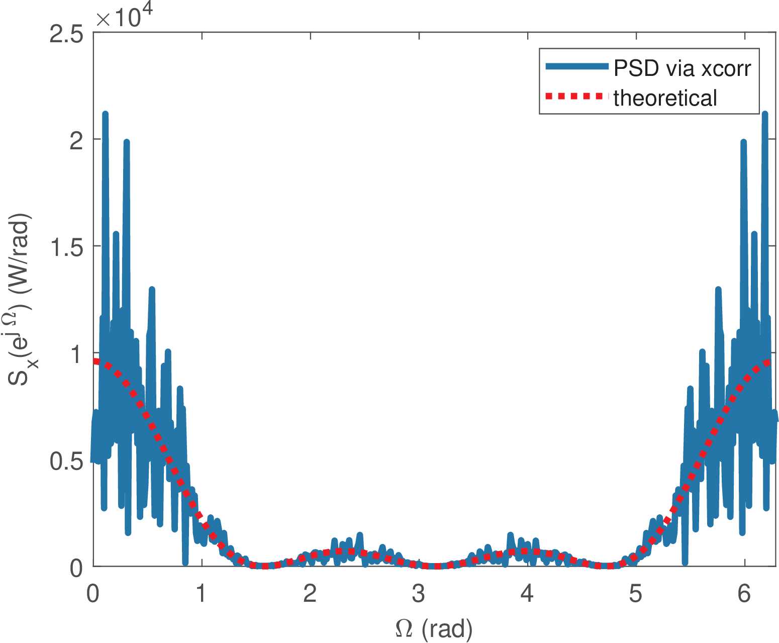
Note that for an input signal with $N$ samples, the function xcorr would, by default, output an autocorrelation with lags from $- N$ to $N$ . However, to avoid noisy estimations at the autocorrelation tails, it is a good strategy to use a maximum lag $M « N$ , if possible. There is a rule of thumb that suggests adopting $M = N ∕ 10$ . This was used in Listing 4.16, where Ry was calculated for a maximum lag of M=256 while the signal had N=3000 samples. $□$

Example 4.19. PSD of a discrete-time impulse. Let $x [n] = Aδ [n - n_{0}]$ be a discrete-time impulse with amplitude $A$ that is multiplied by a rectangular window of $N$ samples for FFT-based spectral analysis. For example, with $N = 5$ and $A = 6$ and x=[6, 0, 0, 0, 0] is the vector representing $x_{w} [n]$ . Because the PSD disregards the phase information, the value of $n_{0}$ and the position of the peak with amplitude $A$ within the windowed signal $x_{w} [n]$ is not relevant. For the given example, using x=[0, 0, 0, 6, 0] would lead to the same results. This signal $x_{w} [n]$ also has an autocorrelation that is an impulse. And its PSD is white with a constant value of $S (e^{j Ω}) = P = 36 ∕ 5 = 7.2$ , as indicated in Eq. (4.44). One can interpret the density $7.2 ∕ (2 π)$ in units of W/rad. Listing 4.17 calculates the periodogram and MS spectrum.

Listing 4.17: MatlabOctaveCodeSnippets/snip_frequency_impulse_PSD.m. [ Python version]

1N=5; %number of FFT points 
2M=2; %maximum number of autocorrelation lags 
3BW=1; %bandwidth 
4x=[6 0 0 0 0]; %impulse signal truncated in N samples 
5Sms=abs(fft(x)/N).^2 %MS spectrum: all values are 2.25 Watts 
6Sk=periodogram(x,[],length(x),1,'twosided') %periodogram 
7[R,lags]=xcorr(x,M,'biased'); %estimating autocorrelation 
8Sxcorr=abs(fft(R)); %PSD via autocorrelation 
9Power=sum(Sms) %power (7.2 W) obtained from MS spectrum 
10Power2=(BW/N)*sum(Sk) %power (7.2 W) from periodogram 
11Power3=(BW/N)*sum(Sxcorr) %power (7.2 W) from periodogram via xcorr

The last commands obtain the average power equal to 7.2 W using three distinct alternatives. All elements of Sms have a value of $7.2 ∕ 5 = 1.44$ W, given that the power was uniformly distributed over the five discrete frequency values. The bilateral periodogram was calculated assuming a bandwidth $BW = 1$ such that the returned value has all values equal to 7.2, coinciding with $S (e^{j Ω}) = 7.2$ (see Eq. (4.52)). $□$