Power spectral density (PSD)

4.5 Power spectral density (PSD)

In most cases, the signal under analysis has infinite energy, such as a deterministic power signal (e. g. a periodic signal) or realizations of a stationary random process. Therefore, the main interest in spectral analysis relies not on the ESD but on the PSD.

4.5.1 Main property of a PSD

A PSD describes the distribution of power over frequency. The frequency can be linear $f$ in Hz, angular frequency $ω$ in radians/s or discrete-time angular frequency $Ω$ , which is an angle in radians.

Before detailing PSD definitions, this subsection presents their main property: the PSD has the important property that the average power $P$ can be obtained in continuous-time by

P_{c} = \int_{- \infty}^{\infty} S (f) d f,

(4.20)

with $S (f)$ in watts/Hz.

Similar to the reasoning associated to Eq. (4.19), the version of Eq. (4.20) when the continuous-time PSD $S (ω)$ is a function of $ω = 2 πf$ in radians/s is

P_{c} = \frac{1}{2 π} \int_{- \infty}^{\infty} S (ω) d ω,

(4.21)

and $S (ω) ∕ (2 π)$ is interpreted in units of watts per rad/s.

The PSD definition in discrete-time is

P_{d} = \frac{1}{2 π} \int_{< 2 π >} S (e^{j Ω}) d Ω,

(4.22)

where $S (e^{j Ω}) ∕ (2 π)$ is interpreted in units of watts per radians.

Table 4.3 summarizes the discussed PSD functions.

Table 4.3: PSD functions.

P

is the average power and the column “Ind. var.” indicates the units and symbols used for the independent variable of each function.

F_{f}

and

F_{ω}

denote the Fourier transform in Hertz and rad/s, respectively. The units of

S (f)

S (ω) ∕ (2 π)

and

S (e^{j Ω}) ∕ (2 π)

are W/Hz, W/(rad/s) and W/rad, respectively.


Time	Ind. var.	Definition	Main property

Continuous-time	$f$ (Hz)	$S (f) = F_{f} {R (τ)}$	$P = \int_{- \infty}^{\infty} S (f) d f$

Continuous-time	$ω$ (rad/s)	$S (ω) = F_{ω} {R (τ)}$	$P = \frac{1}{2 π} \int_{- \infty}^{\infty} S (ω) d ω$

Discrete-time	$Ω$ (rad)	$S (e^{j Ω}) = F {R [ℓ]}$	$P = \frac{1}{2 π} \int_{< 2 π >} S (e^{j Ω}) d Ω$

4.5.2 PSD definitions

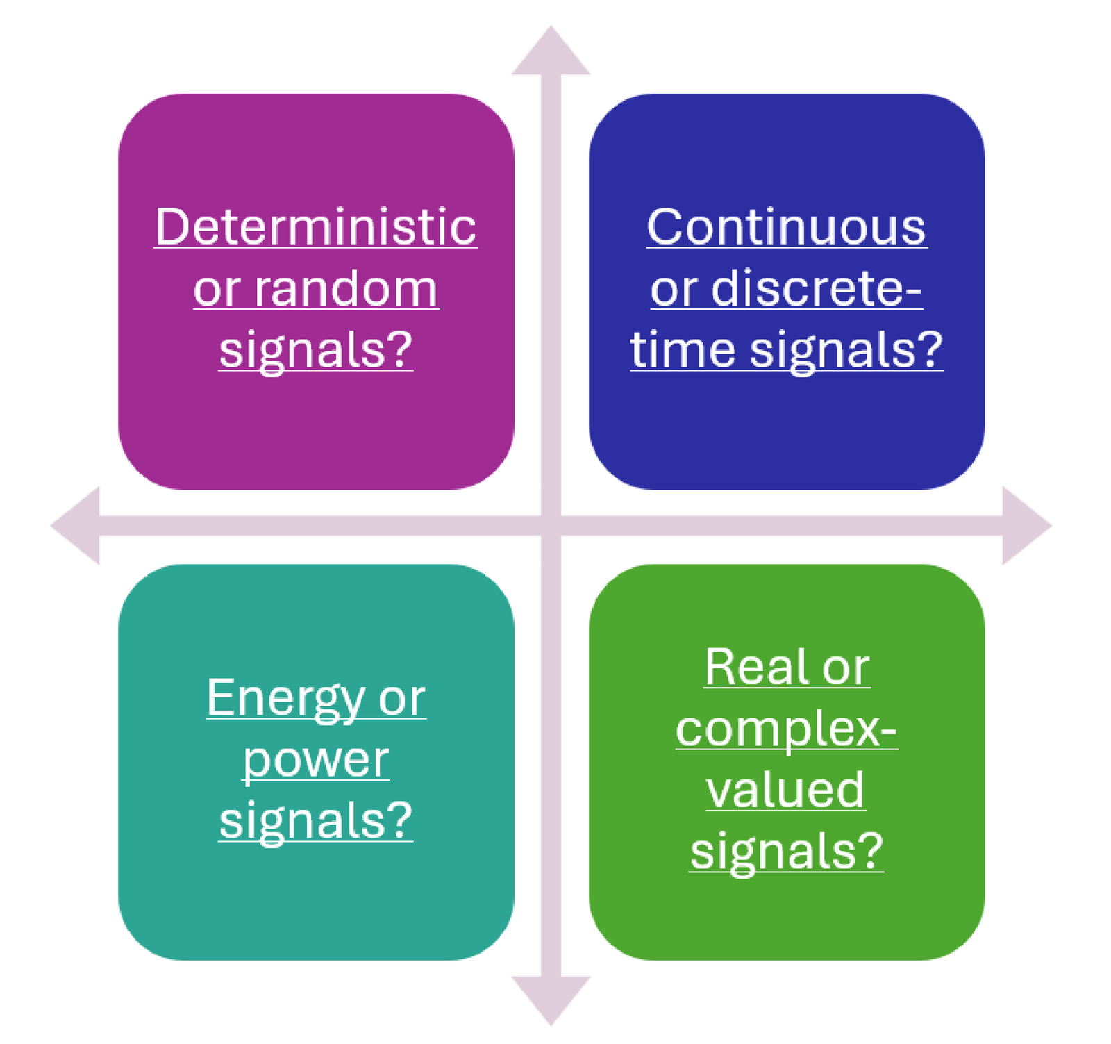
As discussed in Section 1.6, there are many categories of signals. Figure 4.24 illustrates some of them.

Figure 4.24: Important categories of signals. Some of these features need to be taken in account when defining the PSD function.

Similar to the definitions of correlation in Table 1.9, different categories of signals require distinct definitions of PSD. To simplify the discussion, some spectral analysis textbooks⁴ choose to emphasize discrete-time random signals, and define the PSD for this kind of signals. Moreover, the spectral estimation problem is defined in these textbooks⁵ as:

From a finite-length record ${y [1], \dots, y [N]}$ of a second-order stationary random process, find an estimate $Ŝ (e^{j Ω})$ of its power spectral density $S (e^{j Ω})$ for $Ω \in [- π, π]$ .

In other words, the context of this specific problem is restricted to discrete-time power signals with duration of $N$ samples. Here we also discuss other cases, such as: a) continuous-time PSDs, b) when the signal is deterministic and c) the theoretical PSD expressions for infinite-duration signals. This will require attention to adopting the correct definitions.

For instance, the PSD $S (f)$ for a continuous-time power signal can be defined as

S (f) = lim_{T \to \infty} \frac{𝔼 [| X_{T} (f) |^{2}]}{T},

(4.23)

where $X_{T} (f)$ is the Fourier transform of a signal obtained by multiplying the original signal by a window of duration $T$ . Alternatively, the PSD definition for continuous-time deterministic signals is

S (f) = lim_{T \to \infty} \frac{| X_{T} (f) |^{2}}{T},

which is basically the ESD normalized by the time interval $T$ .

An important method for obtaining the PSD of a wide-sense stationary (WSS) random process is given by the Wiener–Khinchin theorem,⁶ which states that the PSD is the Fourier transform of the autocorrelation function.

For instance, assuming $R (τ)$ is the autocorrelation of a WSS random process $X (t)$ , the PSD can be obtained via

S (f) = F {R (τ)} .

(4.24)

Analogous results hold in the discrete-time case, where the PSD is the DTFT of the autocorrelation sequence:

S (e^{j Ω}) = ∑_{ℓ = - \infty}^{\infty} R [ℓ] e^{- j Ω ℓ},

(4.25)

where $ℓ \in ℤ$ is the lag, and the inverse DTFT gives

R [ℓ] = \frac{1}{2 π} \int_{- π}^{π} S (e^{j Ω}) e^{j Ω ℓ} d Ω .

(4.26)

Similar constructions apply to deterministic finite-energy signals, where the ESD is the Fourier transform of the signal’s autocorrelation function. The next subsections provide more details about distinct PSD definitions.

4.5.3 Advanced: PSD of random signals

It makes complete sense to focus the study of PSD estimation on random signals, because they are important in many applications, such as in digital communications. One useful model for these signals is the wide-sense stationary (WSS) random process with autocorrelation $R (τ)$ (see definitions in Appendix A.20). In many spectral analysis problems,⁷ besides being WSS, the random process is assumed to be autocorrelation ergodic.⁸

The PSD $S (f)$ for a continuous-time power signal $x (t)$ corresponding to a realization of a WSS stochastic process $X (t)$ is defined as

S (f) \overset{def}{=} lim_{T \to \infty} \frac{𝔼 [| X_{T} (f) |^{2}]}{T},

(4.27)

where $X_{T} (f)$ is the Fourier transform of a truncated (windowed) version of $x (t)$ with duration $T$ . In other words, $X_{T} (f) = F {x_{T} (t)}$ where $x_{T} (t) = x (t)$ for $- T ∕ 2 \leq t \leq T ∕ 2$ or zero otherwise.

Similar to Eq. (4.27), the PSD $S (e^{j Ω})$ for a discrete-time power signal $x [n]$ corresponding to a realization of a WSS stochastic process $X [n]$ is defined as

S (e^{j Ω}) \overset{def}{=} lim_{N \to \infty} \frac{1}{N} 𝔼 [{| \sum_{n = 0}^{N - 1} x [n] e^{- j Ω n} |}^{2}] = lim_{N \to \infty} \frac{1}{N} 𝔼 [{| X_{N} (e^{j Ω}) |}^{2}] .

(4.28)

where $X_{N} (e^{j Ω})$ is the DTFT of $x_{N} [n]$ , a truncated version of $x [n]$ obtained via a rectangular window of $N$ non-zero samples. The unit of $S (e^{j Ω}) ∕ (2 π)$ is watts per radians.

In practice, there is a finite number of realizations of $X [n]$ and often only one realization $x [n]$ is available. Fortunately, ergodicity of the autocorrelation can be assumed in many cases and the ensemble averages substituted by averages taken over time (see Appendix A.19). Besides, the number of samples (the duration of $x [n]$ ) is often limited to a given value that can be determined, for example, by the time over which the process can be considered stationary. For example, in speech analysis applications, it is typically assumed the process of vowel production is quasi-stationary over segments with durations from 40 to 80 ms. With limited-duration signals, the challenge for spectral analysis is to obtain accurate estimates, as discussed in this chapter.

For both Eq. (4.27) and Eq. (4.28), windows other than the rectangular can be used when the signal under analysis has a short duration. But a rectangular window with infinite duration is the adequate window for the PSD definition.

4.5.4 Advanced: PSD of deterministic and periodic signals

Noticing from Eq. (4.15) and (4.18) that squared magnitudes of $X (f)$ provide the energy distribution over frequency, to obtain the power distribution one can intuitively consider dividing the ESD by “time”, via a normalization factor that converts energy into power.

The PSD definition that is adopted for continuous-time deterministic signals (and does not require the expected value used in Eq. (4.27)) is

S (f) = lim_{T \to \infty} \frac{| X_{T} (f) |^{2}}{T},

which is basically the ESD normalized by the time interval $T$ .

A special case of deterministic signals are the periodic ones. Assuming a continuous-time signal $x (t)$ with period $T_{0}$ , its PSD is

S (f) = \sum_{k = - \infty}^{\infty} | c_{k} |^{2} δ (f - k F_{0}),

(4.29)

where $c_{k}$ are the Fourier Series coefficients and $F_{0} = 1 ∕ T_{0}$ is the fundamental frequency. Similarly, for $S (ω)$ , the expression is

S (ω) = 2 π \sum_{k = - \infty}^{\infty} | c_{k} |^{2} δ (f - k ω_{0}),

(4.30)

where $ω_{0} = (2 π) ∕ T_{0}$ rad/s.

In summary, the PSD $S (f)$ of a deterministic (non-random) periodic signal is composed by impulses with areas determined by the squared magnitude of Fourier series coefficients.

Example 4.9. PSD of a continuous-time sinusoid. If $x (t) = A cos (2 π f_{c} t)$ , then $S (f) = \frac{A^{2}}{4} [δ (f + f_{c}) + δ (f - f_{c})]$ and the average power is $\int_{- \infty}^{\infty} S (f) d f = A^{2} ∕ 2$ . $□$

When considering a discrete-time periodic signal $x [n]$ , its PSD $S (e^{j Ω})$ can be obtained by first considering an expression $S' (e^{j Ω})$ for the frequency range $[0, 2 π [$ :

S' (e^{j Ω}) = 2 π ∑_{k = 0}^{N_{0} - 1} | \tilde{X} [k] |^{2} δ (Ω - k Ω_{0}),

(4.31)

where $N_{0}$ is the period, $Ω_{0} = (2 π) ∕ N_{0}$ is the fundamental frequency, and $\tilde{X} [k]$ the DTFS of $x [n]$ . Finally, the PSD $S (e^{j Ω})$ is simply the periodic repetition of $S' (e^{j Ω})$ :

S (e^{j Ω}) = ∑_{p = - \infty}^{\infty} S' (e^{j (Ω + p 2 π)}) .

(4.32)

Example 4.10. PSD of a discrete-time sinusoid. If $x [n] = A cos (Ω_{1} n)$ (assume $Ω_{1}$ obeys Eq. (1.21) to have $x [n]$ periodic), then $S' (e^{j Ω}) = \frac{π A^{2}}{2} [δ (Ω + Ω_{1}) + δ (Ω - Ω_{1})]$ and

S (e^{j Ω}) = ∑_{p = - \infty}^{\infty} \frac{π A^{2}}{2} [δ (Ω + Ω_{1} + p 2 π) + δ (Ω - Ω_{1} + p 2 π)]

provides its PSD, which has period $2 π$ , as expected. $□$

4.5.5 Advanced: Fourier modulation theorem applied to PSDs

If $S_{x} (f)$ is the PSD of a WSS random process $X (t)$ , the PSD $S_{y} (f)$ of a new process $Y (t) = X (t) e^{j 2 π f_{c} t}$ is

S_{y} (f) = S_{x} (f - f_{c}) .

(4.33)

Similarly, if $Y (t) = X (t) cos (2 π f_{c} t)$ , then

S_{y} (f) = \frac{1}{4} [S_{x} (f + f_{c}) + S_{x} (f - f_{c})] .

(4.34)

To observe why Eq. (4.33) (and, consequently, Eq. (4.34)) is true, recall the Wiener-Khinchin theorem of Eq. (4.24) and the autocorrelation definition of Eq. (1.50). Generally speaking, when modifying a WSS process $X (t)$ , the effect on its PSD can be obtained by checking how the modification affects its autocorrelation, and then relating this to frequency domain using Eq. (4.24). For example, multiplying $X (t)$ by a scalar $α$ corresponds to scaling its autocorrelation $R_{x} (τ)$ by $α^{2}$ and leads to a PSD $α^{2} S_{x} (f)$ given the linearity of the Fourier transform.

According to this reasoning, a proof sketch of Eq. (4.33) follows:

\begin{array}{l} S_{y} (f) & = F {R_{y} (τ)} \\ = F {𝔼 [Y (t + τ) Y^{*} (t)]} \\ = F {𝔼 [X (t + τ) e^{j 2 π f_{c} (t + τ)} X^{*} (t) e^{- j 2 π f_{c} t}]} \\ = F {e^{j 2 π f_{c} τ} 𝔼 [X (t + τ) X^{*} (t)]} \\ = F {e^{j 2 π f_{c} τ} R_{x} (τ)} \\ = S_{x} (f - f_{c}) . \end{array}

Eq. (4.34) can be obtained by decomposing the cosine $cos (2 π f_{c} t) = 1 ∕ 2 (e^{j 2 π f_{c} t} + e^{- j 2 π f_{c} t})$ into two complex exponentials and taking in account that the factor $α = 1 ∕ 2$ leads to the $1 ∕ 4$ in the PSD expression. Eq. (4.34) allows to observe that the result of a signal multiplied by a cosine of unitary amplitude has half of the original signal power.

⁴ For instance, see [Hay09, SM05].

⁵ See [SM05], page 13.

⁶ See, e. g. [ url3wie] and note that a realization $x (t)$ of a WSS process $X (t)$ is not square integrable and does not have a Fourier transform.

⁷ See [Hay09], page 391, Chapter 8.

⁸ An autocorrelation ergodic process is a stochastic process for which time averages of autocorrelation converge to their ensemble averages, allowing the autocorrelation to be estimated from a single realization.