Nonparametric PSD Estimation via Welch’s method

4.7 Nonparametric PSD Estimation via Welch’s method

This section discusses Welch’s method, one of the most popular nonparametric PSD estimation method.

4.7.1 The periodogram variance does not decrease with N

It may seem counterintuitive but, as Figure 4.34 indicates, increasing the number $N$ of samples does not decrease the variance of the periodogram estimates $Ŝ [k]$ .

In fact, it is well-known in spectral analysis theory⁹ that the periodogram $Ŝ [k]$ is an unbiased estimator of the true PSD $S (f)$ , i. e.,

lim_{N \to \infty} 𝔼 [Ŝ [k]] = S (f) .

In other words, the average periodogram converges to the right values as $N$ increases.

However, the variance of the periodogram estimator is approximately $S^{2} (f)$ even for large $N$ . This is a consequence of a result that is valid under mild conditions:

𝔼 [{(Ŝ [k] - S (f))}^{2}] = S^{2} (f) + R_{N},

(4.54)

where $R_{N}$ tends to zero when $N \to \infty$ . In other words, the standard deviation of the periodogram is approximately as large as the spectrum it should estimate. Using windows such as Hamming and Hann can improve the spectral analysis, but does not help with respect to the variance of the periodogram.

One may expect that increasing the number $N$ of samples would lead to a better estimate of the PSD. In fact, the estimation does improve, but with respect to its frequency resolution $Δ f = F_{s} ∕ N$ , not the variance.

4.7.2 Welch’s method for PSD estimation

The main strategy to decrease the variance of a PSD estimation is to split the available data into $K$ segments of $M$ samples each, calculate the periodogram for each segment and then take their average. Methods such as Bartlett’s and Welch’s are based on this principle. The disadvantage of using less ( $M < N$ ) samples is that the frequency resolution $Δ f$ decreases (from $Δ f = F_{s} ∕ N$ to $F_{s} ∕ M$ ).

The main distinction between Bartlett’s and Welch’s methods is that the latter tries to combat the decrease in $Δ f$ by overlapping segments, such that for a given $K$ , the value of $M$ can be larger than $M = N ∕ K$ , where $N$ is the total number of available samples. For example, an overlap of 50% of segments of length $M = 4$ means that the first segment corresponds to samples with indices $n = 0, 1, 2, 3$ , the second segment has samples with $n = 2, 3, 4, 5$ , the third with $n = 4, 5, 6, 7$ and so on.

In Matlab/Octave, the command Sx=pwelch(x) estimates a PSD via Welch’s method using default values ( $K = 8$ , Hamming window and an overlap of 50%). An example of a complete command is

1[Sx,w] = pwelch(x,window,Num_overlap,N_fft,Fs,'twosided')

where window is the window, Num_overlap is the number of samples that are shared between two neighboring segments, N_fft is the number $N$ of FFT points used for calculating the periodograms, Fs is the sampling frequency and ’twosided’ can be used to force pwelch to return values from 0 to $2 π$ , even if the signal is real. The number $M$ of samples per segment corresponds to the window length. The companion function ak_psd.m illustrates how to invoke pwelch.m and is convenient when the sampling frequency is given in Hz.

Figure 4.36: PSD of a white noise $x [n]$ with power equal to 600 W estimated by Welch’s method with $M = 32$ (top) and $M = 256$ (bottom) samples per segment.

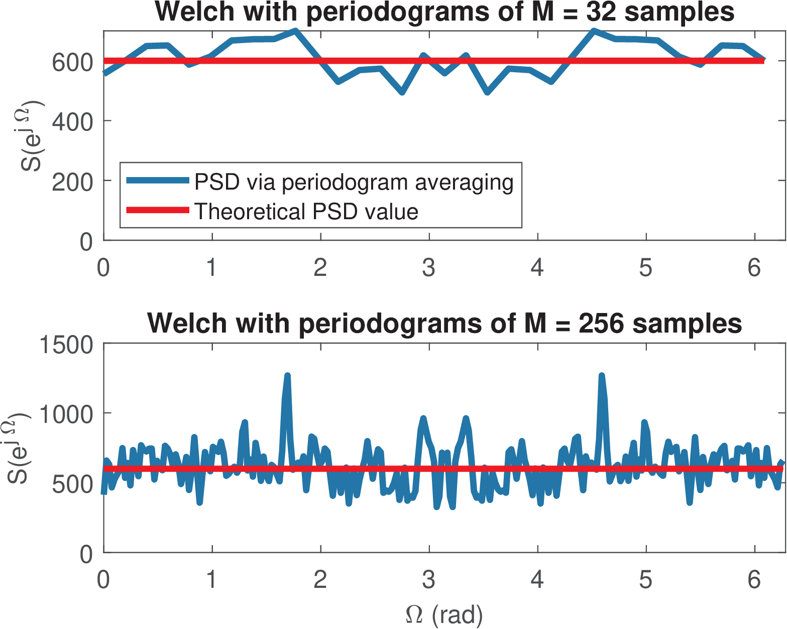
Example 4.20. Variance reduction with Welch’s method. Listing 4.18 provides an example of using pwelch for PSD estimation of the same signal as Figure 4.34 and leads to Figure 4.36. The top plot was obtained with Nfft=32 and then, the code was modified to use Nfft=256 and generate the bottom plot. Note that the total number of samples is N=3000 in both cases. The standard deviations among the periodograms were 46.5 and 132.0, respectively. The smaller Nfft, a larger number of periodograms is calculated and their averaging reduces the variance.

Listing 4.18: MatlabOctaveCodeSnippets/snip_frequency_pwelch.m. [ Python version]

1N = 3000; %total number of signal samples 
2Nfft = 32; %segment length M and also FFT-length 
3Fs = 1; %assumed bandwidth for discrete-time signal 
4power_x = 600; %noise power in Watts 
5x=sqrt(power_x) * randn(1,N); %Gaussian white noise 
6[Sk,F]=pwelch(x,hamming(Nfft),[],Nfft,Fs,'twosided'); %Parameter [] 
7%is because in Matlab it is num. samples while Octave is percent (%) 
8disp(['Periodogram standard deviation=' num2str(std(Sk))]) 
9plot(2*pi*F,Sk) %periodogram with Fs=1 is discrete-time PSD 
10hold on, plot(w,power_x*ones(1,length(w)),'r') %PSD theoretical value

When comparing the plots in Figure 4.36 with the bottom plot in Figure 4.34, which also used $N = 3000$ samples, it is evident that averaging periodograms (for example, via Welch’s method) decreases the variance. Figure 4.36 also illustrates the tradeoff between variance reduction and frequency resolution as the top graph with $Δ Ω = 2 π ∕ 32$ is much smoother than the bottom one with $Δ Ω = 2 π ∕ 256$ .

A detail is that Listing 4.18 uses the default of the window overlap (the third argument of pwelch.m as []) because Octave assumes it is a percentage while Matlab assumes it is the number of samples. $□$

Example 4.21. Estimating the PSD of filtered white noise via Welch’s method.

Figure 4.37: PSD of a filtered white noise $x [n]$ estimated by Welch’s method.

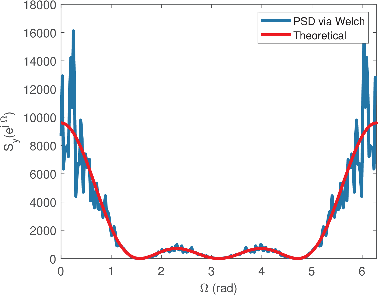
Listing 4.19 illustrates an application of $S_{y} (e^{j Ω}) = σ_{x}^{2} | H (e^{j Ω}) |^{2}$ (Eq. (4.45)), where the system impulse response is h=[1,1,1,1] and $H (e^{j Ω})$ is a sinc.

Listing 4.19: MatlabOctaveCodeSnippets/snip_frequency_filtered_noise_PSD.m

1N = 3000; %total number of signal samples 
2L = 4; %number of non-zero samples of h[n] 
3power_x = 600; %noise power in Watts 
4x=sqrt(power_x) * randn(1,N); %Gaussian white noise 
5h=ones(1,L); %shaping pulse with square waveform 
6y=conv(h,x); %filter signal x with filter 
7Nfft = 256; %segment length M and also FFT dimension 
8Fs = 2*pi; %sampling frequency for discrete-time PSD 
9[Sy_pwelch,w]=pwelch(y,hamming(Nfft),[],Nfft,Fs,'twosided'); 
10H=fft(h,4*N); %DTFT (sampled) of the impulse response 
11Sy_th=power_x*abs(H).^2; %PSD theoretical expression 
12plot(w,2*pi*Sy_pwelch); hold on %scale by 2*pi to get disc.time PSD 
13plot(linspace(0,2*pi,length(H)),power_x*abs(H).^2,'r')

Listing 4.19 was used to generate Figure 4.37, where one can notice that, even with the averaging used in pwelch, the variance continues proportional to the PSD magnitude, as indicated by Eq. (4.54). $□$

Example 4.22. Welch’s method using the Goertzel algorithm. Note that in Matlab, when the call to pwelch specifies the frequency points, pwelch can use the Goertzel algorithm instead of an FFT. An example is the following code:

1x=randn(1,10000); Fs=1e4; %some random vector and sampling freq. 
2f=linspace(-Fs/2,Fs/2,1024); %create a frequency axis 
3Px=pwelch(x,hamming(1024),512,f,Fs); %Octave has distinct syntax! 
4plot(f,10*log10(Px)); %show PSD from -Fs/2 to Fs/2

The Goertzel algorithm can slow down the computations when compared to the FFT-based PSD estimation because it targets situations in which the frequencies are not uniformly spaced such as in DTMF detection algorithms (see Figure 4.50). $□$

⁹ See, e. g., [Hay96, SM05] and [ url4spe].