Extra Exercises

4.13 Extra Exercises

4.1. Taking Figure 4.34 as a reference, decode the DTMF symbols of Figure 4.46, which correspond to a phone number with eight digits.

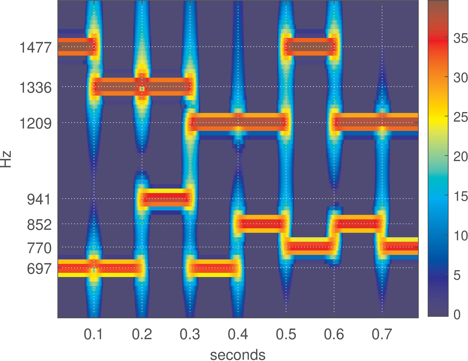
Figure 4.46: Eight DTMF symbols, each one with a 100 ms duration.

4.2. Can a discrete-time random process

X [n]

have infinite power? If yes, under what conditions? Can these conditions be achieved in practice?
4.3. Modify Listing 4.35 to investigate how the sidelobes are decreased in the DTFT of the Hann window by combining three DTFTs of a rectangular window. Then, perform the same analysis for the Hamming window.

Listing 4.35: MatlabOctaveCodeSnippets/snip_frequency_testHannDTFT.m

1function snip_frequency_testHannDTFT 
2N=9; %number of window samples 
3[dtftHann,w]=freqz(hann(N)); %get values of the DTFT as reference 
4dtftHann2=0.5*rectWinDTFT(w,N)- 0.25*rectWinDTFT(w+(2*pi/(N-1)),N)... 
5    -0.25*rectWinDTFT(w-(2*pi/(N-1)),N); %DTFT using expression 
6plot(w,real(dtftHann-dtftHann2),w,imag(dtftHann-dtftHann2)) %error 
7end 
8function D=rectWinDTFT(w,N) %get DTFT of rectangular window 
9D=sin(0.5*N*w)./sin(0.5*w).*exp(-j*0.5*w*(N-1)); 
10end

4.4. Explore the computation and relationships among convolution, correlation and FFT. Assume a vector x=[0 1 4 8 0] with

M = 5

elements. a) Explain why in Matlab, conv(x,x), the convolution of x with x itself results into a vector with

2 M - 1

elements. b) Compare the equation of a convolution x[n]

*

h[n]

y [n] = \sum_{k = - \infty}^{\infty} h [k] x [k - n]

with the equation of an autocorrelation

R [ℓ] = \sum_{k = - \infty}^{\infty} x [k] x [k + ℓ] .

Then, prove that x[n] $*$ x[ $-$ n]=R[n] and confirm it in Matlab observing that conv(x,fliplr(x)) and xcorr(x) lead to (approximately) the same result in Matlab. Plot conv(x,x) and xcorr(x). c) The results differ in b) mainly because xcorr uses a FFT to compute the correlation. Try to explain how the following code is used to compute the autocorrelation

    % Autocorrelation
    % Compute correlation via FFT
    X = fft(x,2^nextpow2(2*M-1));
    c = ifft(abs(X).^2);

You may want to use type xcorr and take a look at the source code to see how the vector c above is modified to give the expected result (i.e., there is a postprocessing step after the two lines above).
4.5. Short-time energy. Use the same procedure as before to record the sentence “We were away” or similar. Calculate the speech energy $e$ for each frame of $t$ milliseconds (ms), without overlap among frames. Use $t \in {10, 30, 100, 200}$ ms to get four energy trajectories. Estimate the first-derivative of $e$ using $Δ e_{n} = e_{n} - e_{n - 1}$ . Estimate the second-derivative using $Δ Δ e_{n} = Δ e_{n} - Δ e_{n - 1}$ . Use subplot to show simultaneously the waveform (subplot(411)) , $e$ (subplot(412)), $Δ e$ (subplot(413)) and $Δ Δ e$ (subplot(414)). Do that for each $t$ and choose the value of $t$ that leads to the best plots in terms of distinguishing when it is silence or speech.
4.6. Spectrograms. Use a function such as specgram to plot both the wide and narrowband spectrograms of the sentence recorded in the previous exercise. In both cases, a) what were the window lengths and equivalent bandwidths you used? b) What were the complete commands?
4.7. Linear regression. Assume there are $N$ points $(x, y)$ , where $x \in ℝ$ and $y \in ℝ$ . Find the parameters $a$ and $b$ of a first order polynomial $\tilde{y} = ax + b$ that best fits the data in terms of the minimum total squared error $E = \sum_{n = 1}^{N} {(y_{n} - {\tilde{y}}_{n})}^{2}$ . However, try to write the two final equations using correlations (for example, the autocorrelation $R_{x} (0) = \sum_{n = 1}^{N} x_{n}^{2}$ at lag $m = 0$ is one possible term). Use your equations to fit a line to the following training data: x=rand(1,100); y=3*x+4+0.5*randn(1,100); plot(x,y,’x’) and plot the line superimposed to the training data.
4.8. LPC analysis using the autocorrelation method. Assume we want to calculate a LPC filter of order $P = 3$ for the signal $x [n] = (10, 8, 3, - 2, - 4, - 2, 1, 2)$ using the autocorrelation method. The 3-rd order predictor is given by the difference equation

\tilde{y} [n] = a_{1} x [n - 1] + a_{2} x [n - 2] + a_{3} x [n - 3] .

By convention, the LPC filter is given (in the Z-domain) as

A (z) = 1 - a_{1} z^{- 1} + a_{2} z^{- 2} + a_{3} z^{- 3}

and you can get it using lpc(x,3) in Matlab. a) Try to prove that the coefficients $a_{i}$ can be found by solving

[\begin{matrix} R (0) & R (1) & R (2) \\ R (1) & R (0) & R (1) \\ R (2) & R (1) & R (0) \end{matrix}] [\begin{matrix} a_{1} \\ a_{2} \\ a_{3} \end{matrix}] = [\begin{matrix} R (1) \\ R (2) \\ R (3) \end{matrix}]

where $R (m)$ is the correlation at lag $m$ . b) One can note that the matrix in the equation above is symmetric and, besides, has equal elements along the diagonals. This is called a Toeplitz matrix. The matrix can be inverted with the Levinson-Durbin algorithm below, that is $O (P^{2})$ instead of a generic inversion method that is $O (P^{3})$ .

Listing 4.36: MatlabOctaveCodeSnippets/snip_frequency_Levinson_Durbin.m. [ Python version]

1function [a,k,E]=snip_frequency_Levinson_Durbin(R,p) 
2% function [a,k,E]=snip_frequency_Levinson_Durbin(R,p) 
3%Usage: x=randn(1,100)+linspace(1,5,100); p=10; R=xcorr(x,p); 
4%       R=R(p+1:end); %keep only values of interest: R(0)...R(p) 
5%       [a,k,E]=snip_frequency_Levinson_Durbin(R,p) 
6%Inputs: 
7% p - order of LPC analysis 
8% R - p+1 sample correlation function values, R(0)...R(p) 
9%Outputs: 
10% a - p LPC coefficients, from a(1) to a(p) 
11% k - p reflection coefficients, from k(1) to k(p) 
12% E - E energies of error, from E(1) to E(p) 
13%Initialization 
14k(1)=R(1+1)/R(0+1); a(1)=k(1); E(1)=R(0+1)*(1-k(1)^2); 
15%Recursion 
16for i=2:p 
17    k(i)=(R(i+1)-sum(a(1:i-1).*R(i:-1:2)))/E(i-1); 
18    a(i)=k(i); 
19    a(1:i-1)=a(1:i-1)-k(i)*a(i-1:-1:1); 
20    E(i)=E(i-1)*(1-k(i)^2); 
21end

The code above has errors, but it should give the same result as the function levinson in Matlab. For example, levinson([202 114 -2 -68],3) gives the right result, but my_durbin([202 114 -2 -68],3) does not. Unfortunately, levinson is a Mex (compiled) file and one cannot see the code. Consult a reference about LPC and fix the code above.