2.5  Fourier Transforms and Series

The transforms in this section adopt eternal (infinite duration) sinusoids as basis functions and complement the DFT, which uses finite-length basis functions. For mathematical convenience, complex exponentials are also used given that they conveniently represent sinusoids.

Using sinusoids as basis functions is very useful in many applications. Depending on the type of signal to be analyzed, there are four pairs of analysis and synthesis transform equations that adopt eternal sinusoids as basis functions. These four pairs can be collectively called Fourier analysis tools and are discussed in the sequel.

The reason for not having only one transform pair when dealing with Fourier analysis is that two properties of the signal to be analyzed must be taken in account: whether the signal is continuous or discrete in time, and periodic or non-periodic. Covering all possible combinations, Table 2.3 lists the four pairs of equations to conduct Fourier analysis with eternal sinusoids (later we will discuss the DFT, which is used for finite-duration signals).

It can be seen from Table 2.3 that the terminology series is used when the signal to be analyzed is periodic. In this case the spectrum is discrete in frequency and represented by coefficients $c_k$ or $X[k]$. Obtaining a Fourier series is a special case of the general procedure of representing a function (in this case, a periodic signal) via a series expansion such as Taylor’s, Laurent’s, etc. In contrast, the spectrum of non-periodic signals is continuous in frequency and the tools to analyze non-periodic signals are called transforms. Note this nomenclature is not 100% consistent with block transforms in the sense that the DFT, which has a discrete spectrum, is called “transform”.

As highlighted in Table 2.4, in Fourier analysis, there is an interesting and maybe not evident duality between the time and frequency domains: periodicity in one domain leads to a discrete function in the other domain, while non-periodicity leads to a continuous function. For example, Table 2.4 shows that the spectrum of a discrete-time signal $x[n]$ is always periodic.

Table 2.4 and Table 2.3 indicate that the DTFS is the only pair that has discrete signals in both domains, time and frequency. This indicates that the DTFS is related to the DFT. In fact, the DFT and DTFS are mathematically equivalent in case $N_0=N$, with the exception of the normalization factor $1∕N$ in Eq. (2.11). But their interpretation has a remarkable distinction: The basis functions of the block transform DFT in Eq. (2.11) are finite-duration sequences or, equivalently, vectors, with dimension $N$, while the basis functions of the DTFS are infinite-duration complex exponentials $e^{j\frac{2\pi }{N_0}\mathit{kn}}$ of period $N_0$. Hence, the DTFS and DFT are more naturally interpreted and used for (infinite-duration) periodic and finite-duration signals, respectively.

Another reason for keeping their names different is that the DFT (via FFT algorithms) is often used in computers, digital oscilloscopes, spectrum analyzers, etc., to analyze non-periodic and even continuous-time signals that were digitized. Hence, there are aspects that must be studied to apply DFT in these cases, such as the relation between an original spectrum $X(\omega )$ of a continuous-time signal and $X[k]$, the one obtained by the DFT of its discrete-time version. Therefore, in spite of the operations in DTFS and DFT being mathematically equivalent apart from a normalization constant, it is convenient to restrict the discussion of DTFS to the analysis of periodic and discrete-time signals and call DFT the tool for finite-duration signals, which in practice is used for analyzing any digitized signal.

Besides their relation to the DFT, there are many other similarities and relations within the four Fourier pairs in Table 2.4 themselves. For example, transforms are meant for non-periodic signals but, as discussed in Appendix A.26.2, impulses can be used to also represent periodic signals via a transform (instead of a series). The next sections will discuss some of these relations.

One point that will not be explored in this text is the important aspect of convergence. Similar to the fact that a vector outside the span of a given basis set cannot be perfectly represented by the given basis vectors, there are signals that cannot be represented by Fourier transforms or series. In other words, the transform/series may not converge to a perfect representation even when using an infinite number of basis functions. A related aspect is the well-known Gibbs phenomenon: when the signal $x(t)$ has discontinuities (such as $u(t)$ at $t=0$), the Fourier representation has to use an infinite number of basis functions. Any truncation of this number (i. e., using a finite number of basis functions) leads to ripples in the reconstructed signal. Given the adopted emphasis in the engineering application of transforms, this text assumes the signals are well-behaved and the transforms and series properly converge.

Complementing Table 2.3, Table 2.5 indicates the assumed units when the signals in time domain are given in volts and is useful to observe the difference for continuous and discrete spectra.

2.5.1  Fourier series for continuous-time signals

The Fourier series for a continuous-time signal uses an infinite number of complex harmonic sinusoids $e^{\mathit{jk}{\omega }_{0}t},k\in \mathbb{Z},$ as basis functions. These functions allow to represent any periodic signal $x(t)$ with period $T_0$ (i. e., $x(t)=x(t+T_0),\forall <!--\; FUNCTION\; APPLICATION\; -->t$), where ${\omega }_0=\frac{2\pi }{T_0}=2\pi f_0$ (rad/s). The frequency $f_0$ in Hz (or ${\omega }_0$ in rad/s) is called the fundamental frequency.

Advanced: On the orthogonality of sinusoids

The results in this subsection are useful for proving Fourier pairs. They can be eventually skipped in case the mathematical proofs based on the orthogonality of sinusoids are not of interest at this moment.

Result 2.1. Eternal (infinite-duration) sinusoids at different frequencies are orthogonal. If ${\omega }_1\ne {\omega }_2$, then

Proof: To simplify notation, let ${\omega }_{1}t+{\varphi }_1=\alpha$ and ${\omega }_{2}t+{\varphi }_2=\beta$. From Eq. (A.11):

First let us assume that the interval from $-\infty$ to $\infty$ corresponds to an integer number of periods for both $\text{cos}<!--\; FUNCTION\; APPLICATION\; -->(\alpha -\beta )$ and $\text{cos}<!--\; FUNCTION\; APPLICATION\; -->(\alpha +\beta )$. In this case, it is easy to see that the following result is zero:

unless $\alpha =\beta$ (in this case $\text{cos}<!--\; FUNCTION\; APPLICATION\; -->(\alpha -\beta )=1$). But the astute reader may be concerned that the range$]-\infty ,\infty [$ does not necessarily represent an integer number of periods. In fact, using the reasoning that we adopt for finite-duration signals, we should have the integral interval (recall the concept of commensurate frequencies in Example 1.16) corresponding to a multiple of the periods of $\alpha -\beta$ and $\alpha +\beta$. But things are different when the integral interval has infinite duration. In this case, a sinusoid alternates between positive and negative values, and over an infinite interval, the areas under these positive and negative sections cancel each other out. As a result, the integral converges to zero. In spite of not being rigorously stated, this result is important to understand the proof of the expression for the Fourier transform (see, e. g., Section 2.5.3).    $\text{□}$

Result 2.2. Cosine and sine at the same frequency are orthogonal. Similar to Example 2.1, it can be shown that:

which used Eq. (A.5).   $\text{□}$

The following result is useful when the integration interval is the fundamental period $T_0$ or a multiple of $T_0$.

Result 2.3. Harmonic sinusoids are orthogonal when the inner product (integral) is over a time interval multiple of the fundamental period. If ${\omega }_0=2\pi ∕T_0$ is the fundamental frequency in rad/s and $k\ne m$, then

Proof: Note that the sinusoids are assumed here to be eternal, but the result is also valid in case they have a finite-duration coinciding with the time duration of the integral. From Eq. (A.11):

The cosine with angular frequency $(k+m){\omega }_0$ of the second parcel has a period $T=T_0∕(k+m)$ and its integral over $T_0$ is zero, because $T_0$ is an interval corresponding to an integer number of periods $T$. The same reasoning can be applied to the cosine with angular frequency $(k-m){\omega }_0$ with period $T_0∕|k-m|$, which is especially easy to observe when $k>m$. If $k<m$, because $\text{cos}<!--\; FUNCTION\; APPLICATION\; -->(x)=\text{cos}<!--\; FUNCTION\; APPLICATION\; -->(-x)$, the cosine argument of the first parcel can be changed to $(m-k){\omega }_{0}t+{\varphi }_2-{\varphi }_1$ to help concluding that this integral over $T_0$ is also zero.   $\text{□}$

Result 2.4. On the energy of Fourier basis functions. Example 2.3 proves that the Fourier series basis functions are orthogonal. But they are not orthonormal and the energy over a duration $T_0$ is

which is the normalization factor that will appear in the Fourier series equations, similar to the result for block transforms in Eq. (2.25).    $\text{□}$

Result 2.5. Proof of the Fourier series pair. One can use the reasoning in Theorem 4 (page 2003) to prove the Fourier series equations. Writing the synthesis equation

is similar to $\mathbf{\text{x}}={\sum <!--\; FUNCTION\; APPLICATION\; -->}_{i=1}^N{\alpha }_i{\mathbf{\text{b}}}_i$. Calculating $⟨\mathbf{\text{x}},{\mathbf{\text{b}}}_i⟩$ is therefore equivalent to the inner product between $x(t)$ and the $m$-th basis function $e^{j2\mathit{\pi m}{f}_{0}t}$, which is written as:

(recall from Table 2.2 that $⟨x(t),y(t)⟩=\int x(t)y^{\ast }(t)\mathrm{\text{d}}t$ the inner product is defined with the complex conjugate of the second argument when the signals are complex). Due to the properties of the inner product one can write

The last step is due to the orthogonality of the basis functions:

In summary, the previous steps used the basis functions orthogonality to prove that the analysis equation

corresponds to using the inner product as in Theorem 4 (page 2003), and taking in account that here the basis functions have an energy $T_0$.    $\text{□}$

Fourier series using complex exponentials

Looking at Table 2.3, the basis $b(t)=1,\forall <!--\; FUNCTION\; APPLICATION\; -->t$, corresponding to $k=0$ in a Fourier series, is responsible for representing the DC level of $x(t)$. All other basis functions have a frequency

When $k>1$, frequencies higher than $f_0$ are generated and, consequently, a period $T_k=T_0∕k$ that is smaller than $T_0$. Therefore, all basis functions but the one for $k=0$ are periodic in $T_0$. The frequencies $f_k$ that obey a relation $f_k=k{f}_0$ with respect to a fundamental frequency $f_0$ are called harmonics. The frequency $f_2=2f_0$ is called the second harmonic, $3f_0$ is the third harmonic and so on.

It seems intuitive that Fourier series should not be used to represent non-periodic signals. In fact, the basis functions even depend on the period $T_0$ of the signal to be analyzed. On the other hand, because the signal is periodic, it suffices to find coefficients that represent the signal $x(t)$ during a single period. The trick is then to use these coefficients (obtained with inner products of duration $T_0$) to multiply eternal complex exponentials and properly represent the periodic (and consequently infinite-duration) $x(t)$. Hence, the Fourier series pair is:

The negative frequencies $f_k,k=-\infty ,\dots ,-2,-1$ exist for mathematical convenience. They allow, for example, to represent a cosine as a sum of complex exponentials with “positive” and “negative” frequencies as in Eq. (A.2).

(a) $k=0$ (DC)

(b) $k=1$ (fundamental)

(c) $k=2$

(d) $k=-2$

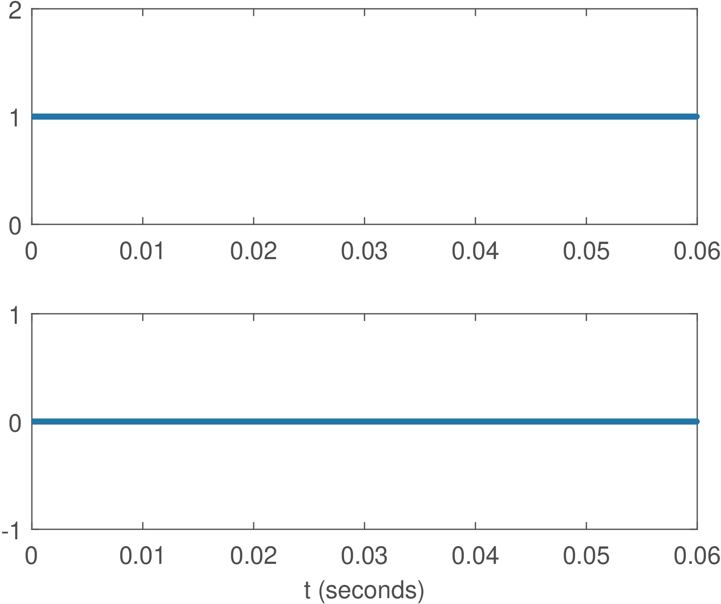
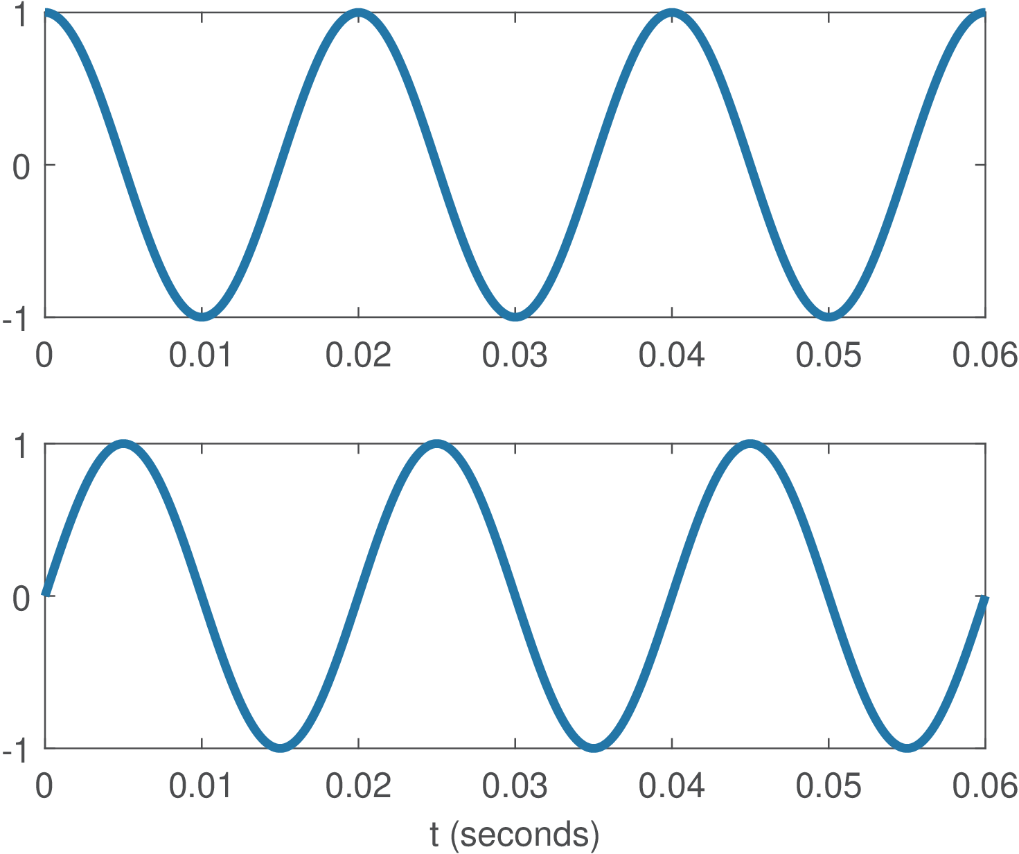
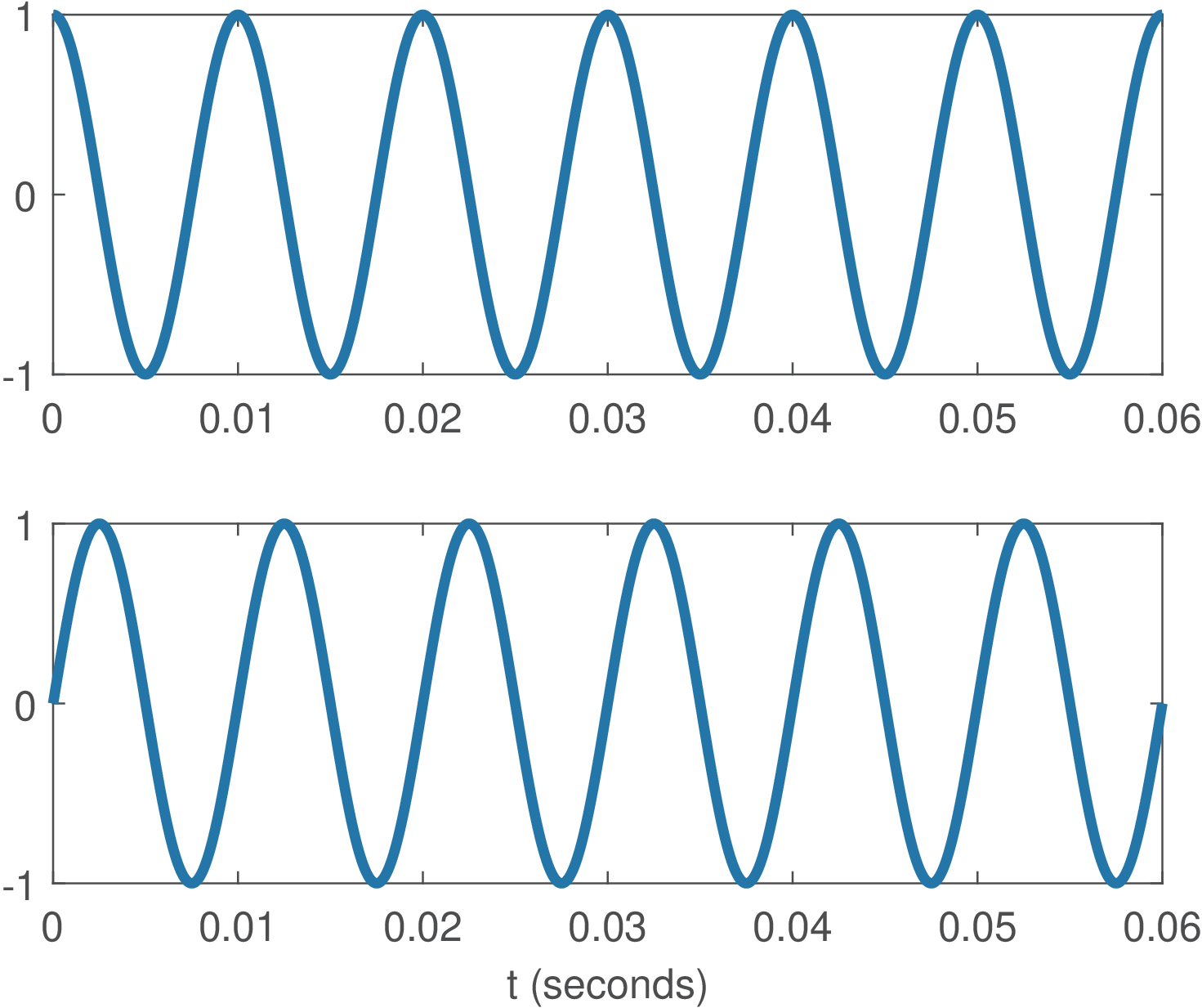
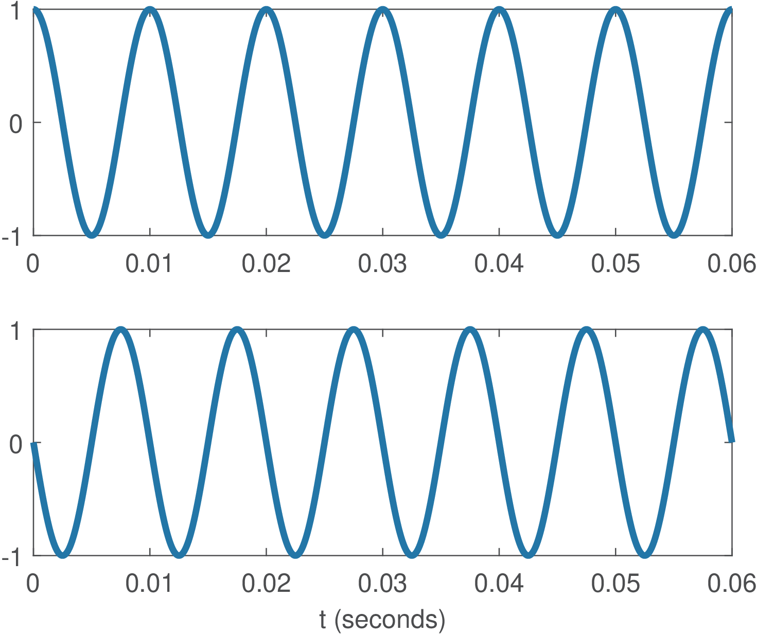
Example 2.14. Basis functions of Fourier series. Figure 2.11 shows four basis functions for analyzing signals with period $T_0=1∕50=0.02$ seconds. Note that the basis for $k=0$ is a real signal while the others are complex. The basis for $k=2$ has the same real part of the one for $k=-2$ and the negative of the imaginary part. This is due to the fact that cosines are even functions $\text{cos}<!--\; FUNCTION\; APPLICATION\; -->(x)=\text{cos}<!--\; FUNCTION\; APPLICATION\; -->(-x)$ while sines are odd functions $\text{sin}<!--\; FUNCTION\; APPLICATION\; -->(x)=-\text{sin}<!--\; FUNCTION\; APPLICATION\; -->(-x)$ (see Section 1.6.1).   $\text{□}$

Similar to the DFT case discussed in Section 2.4.3.0, when the Fourier series is used to analyze a real signal $x(t)$, the symmetry of the basis functions for $k$ and $-k$ leads to interesting properties for the coefficients: the real part of $c_k$ and their magnitude compose even sequences while the imaginary part and their phase compose odd sequences. In summary, for real signals $x(t)$: $|c_k|=|c_{-k}|$, $R\mathit{eal}\{c_k\}=R\mathit{eal}\{c_{-k}\}$, $\angle c_k=-\angle c_{-k}$ and $I\mathit{mag}\{c_k\}=-I\mathit{mag}\{c_{-k}\}$. These properties can be written compactly as

which corresponds to Hermitian symmetry for the Fourier series, as for the DFT in Section 2.4.3.0. In fact, the properties based on the symmetry of the basis functions and, eventually, also of the signal to be analyzed ($x(t)$ in this case), are valid not only for Eq. (2.27) but for other Fourier pairs.

Another aspect due to the symmetry is often invoked: because any signal $x(t)$ can be decomposed as the sum $x(t)=x_e(t)+x_o(t)$ of an even part $x_e(t)$ and an odd part $x_o(t)$ (see Section 1.6.1), the cosines are in charge of representing $x_e(t)$, while the sines represent $x_o(t)$. This leads to conclusions such as: if $x(t)$ is real and even, then $\angle c_k=I\mathit{mag}\{c_k\}=0,\forall <!--\; FUNCTION\; APPLICATION\; -->k$.

Figure 2.12 shows the Fourier coefficients for the periodic and real-valued signal $x(t)=4+10\text{cos}<!--\; FUNCTION\; APPLICATION\; -->(2\pi 50t+2)+4\text{sin}<!--\; FUNCTION\; APPLICATION\; -->(2\pi 150t-1)$, with fundamental period $T_0=1∕f_0=1∕50=0.02$ s. The graphs in Figure 2.12 are called the spectrum of the signal. Because the coefficients $c_k$ are in general complex numbers, a spectrum is represented using the polar or rectangular form of complex numbers. Figure 2.12 uses the polar format. One can notice that, because $x(t)$ is real, $c_{-k}=c_k^{\ast }$, i. e., the spectrum presents the Hermitian symmetry of Eq. (2.28).

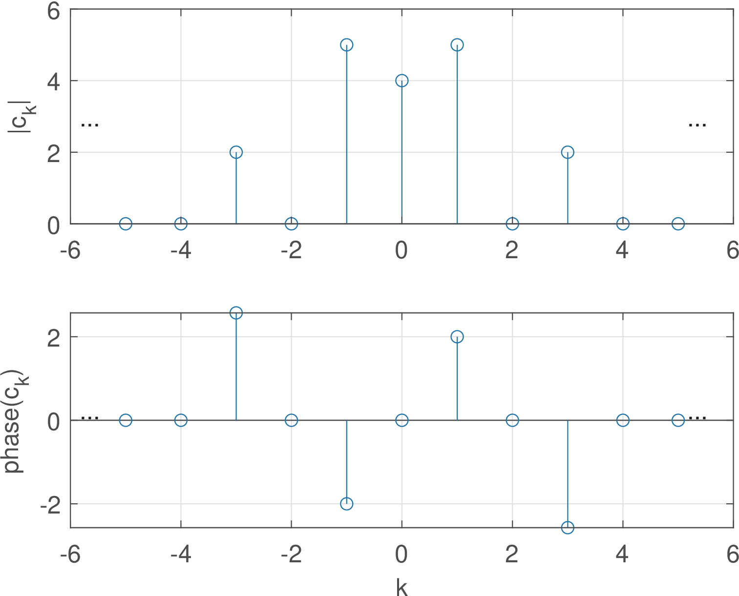
Example 2.15. Continuous-time Fourier series coefficients by inspection. When the periodic signal $x(t)$ is composed by a sum of sines and cosines, it is convenient to obtain the Fourier series coefficients by inspection. For example, assume the signal $x(t)=4+10\text{cos}<!--\; FUNCTION\; APPLICATION\; -->(2\pi 50t+2)+4\text{sin}<!--\; FUNCTION\; APPLICATION\; -->(2\pi 150t-1)$ of Figure 2.12. Using Euler’s, one has

and

Hence, the only non-zero coefficients are $c_0=4$, $c_1=5e^{j2}$, $c_3=2e^{-j(1+\pi ∕2)}$, $c_{-1}=5e^{-j2}$, $c_{-3}=2e^{j(1+\pi ∕2)}$, with $1+\pi ∕2\approx 2.57$ as indicated in Figure 2.12, which shows the magnitude and phase graphs of the Fourier series coefficients for representing $x(t)$.   $\text{□}$

Trigonometric Fourier series

Instead of complex exponentials $e^{\mathit{jk}{\omega }_{0}t}$ with negative frequencies as in Eq. (2.27), the Fourier series can be written in terms of cosines and sines with positive frequencies only. In this case, one has a set of coefficients for the cosines and another set for the sines that are usually called $a_k$ and $b_k$, respectively, and related as follows:

Comparing the expression for $x(t)$ in Eq. (2.27) and Eq. (2.29), they are related via Euler’s formula (see Eq. (A.1)) 

This allows to write $c_0=a_0$ and, for $k>0$:

Eq. (2.29) is called the trigonometric Fourier series while Eq. (2.27) is the exponential version.

Example 2.16. Bilateral and unilateral spectrum representations.

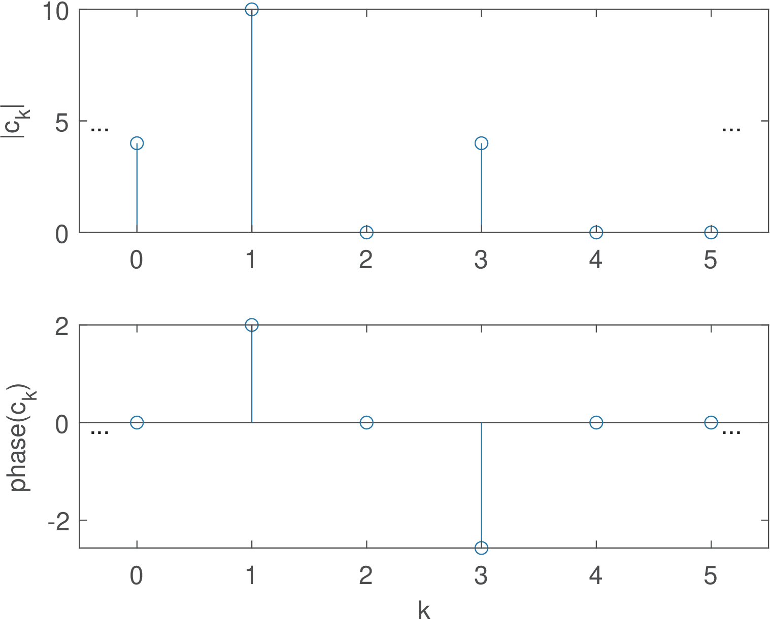
The spectrum of Figure 2.12 is called bilateral because the negative frequencies are explicitly represented. In this case, a sinusoid of amplitude $A$ is represented by a pair of coefficients with magnitudes $A∕2$ each. An alternative representation, valid only for real signals, is the unilateral spectrum, where only $c_k^{\prime },k\ge 0$ are shown. In this case, $c_0^{\prime }=c_0$ and $c_k^{\prime }=2c_k,k>0$ as illustrated in Figure 2.13. This text emphasizes the bilateral representation because it is more general and capable of representing the spectrum of a complex-valued signal $x(t)$.    $\text{□}$

2.5.2  Discrete-time Fourier series (DTFS)

The Fourier series for discrete-time signals is used to analyze a periodic signal $x[n]$ with fundamental period $N_0$. Similar to the continuous-time case, the basis functions consist of a set of complex exponentials formed by a fundamental frequency and its harmonics. The basis corresponding to the fundamental frequency is $e^{j{\mathrm{\Omega }}_{0}n}$, where ${\mathrm{\Omega }}_0=\frac{2\pi }{N_0}$ radians, and the harmonics are ${\mathrm{\Omega }}_k=k{\mathrm{\Omega }}_0$. A major distinction between the DTFS and the Fourier series is that there are only $N_0$ distinct angular frequencies for the DTFS because

This is a consequence of the fact that discrete-time angular frequencies are angles. Hence, the basis function corresponding to a frequency $\mathrm{\Omega }=\pi$ is equal to the one corresponding to $\mathrm{\Omega }=\pi +2\pi =3\pi$.

Hence, the DTFS pair is:

If convenient, Eq. (2.30) can be represented using the twiddle factor $W_{N_0}=e^{-\frac{j2\pi }{N_0}}$ as in Table 2.3. The notation $n=⟨N_0⟩$ and $k=⟨N_0⟩$ represent any interval of $N_0$ consecutive integers, such as $0,1,\dots ,N_0-1$ or $-N_0,-(N_0-1),\dots ,-1$. Note the basis functions depend on the period $N_0$ of the signal to be analyzed.

Because $x[n]$ is periodic, it suffices to specify its samples in an interval $⟨N_0⟩$. However, using $k=-\infty ,\dots ,-1,0,1,\dots ,\infty$ and $n=-\infty ,\dots ,-1,0,1,\dots ,\infty$ in Eq. (2.30) allows to indicate that $X[k]$ is periodic and $x[n]$ has an infinite duration (in contrast to the finite-duration sequence obtained by an inverse DFT), respectively. As indicated in Eq. (2.30), only $k=⟨N_0⟩$ values of $X[k]$ are necessary to represent the periodic $x[n]$, and along $k$ the values $X[k]$ are periodic, i. e., $X[k]=X[k+N_0]$. The reason is that, as mentioned, the angles repeat $(k+N_0){\mathrm{\Omega }}_0=k{\mathrm{\Omega }}_0$ after $N_0$ samples (as also illustrated by the divided unit circle in Figure 2.7) and, consequently, their corresponding basis functions and coefficients $X[k]$.

Similar to Example 2.15, which obtained the Fourier series of a continuous-time signal, when $x[n]$ is composed by a sum of sinusoids, it is relatively easy to find the DTFS coefficients $X[k]$ by inspection, as discussed next.

Example 2.17. DTFS coefficients by inspection. Assume $x[n]=A\text{cos}<!--\; FUNCTION\; APPLICATION\; -->(\frac{\pi }{6}n+\pi ∕3)$, which has a period of $N=12$ samples. Instead of calculating via Eq. (2.30), one can rewrite the signal as a sum of complex exponentials:

With $N=12$, the DTFS synthesis equation is:

where the range $k=⟨12⟩$ is chosen to be: $k=-6,-5,\dots ,0,1,\dots ,5$, which leads to

By inspection, $x[n]$ can be represented by two coefficients: $X[-1]=\frac{A}{2}{e}^{-\mathit{j\pi }∕3}$ and $X[1]=\frac{A}{2}{e}^{\mathit{j\pi }∕3}$, while all other coefficients in the range $k\in [-6,5],k\ne \pm 1$ are zero.

If the range $k=⟨12⟩$ were $k=0,1,\dots ,11$, it would be necessary to recall that $X[k]=X[k+N]$. Hence, $X[11]=X[1]$ and the spectrum of $x[n]$ could be represented by $X[1]=\frac{A}{2}{e}^{\mathit{j\pi }∕3}$ and $X[11]=\frac{A}{2}{e}^{-\mathit{j\pi }∕3}$ with $X[k]=0$ for $k=0$ and $1<k<11$. An alternative view of this periodicity is to sum $2\mathit{\pi n}$ to the angle $e^{-j\frac{\pi }{6}n}$, which leads to $e^{j2\mathit{\pi n}}{e}^{-j\frac{\pi }{6}n}=e^{j\frac{11\pi }{6}n}$ and allows to write

Sometimes the graphs do not emphasize, but DTFS is always periodic and the Fourier coefficients repeat over $k$ with a period $N$.   $\text{□}$

Calculating the DTFS via the DFT

As mentioned, mathematically the DFT and DTFS differ only by the scaling factor $1∕N$, as indicated in Eq. (2.20) and Eq. (2.30), respectively. Using the proper scaling factor will not alter the spectrum shape but it is important in case the numerical values should be interpreted with the correct units. For example, if a cosine is generated and its FFT calculated in Matlab/Octave, the numerical values will be influenced by both the cosine amplitude and value of $N$. Only after the normalization by $1∕N$ one can interpret the spectrum of a periodic signal in volts. The following example illustrates this procedure.

Example 2.18. DTFS using an FFT routine. Having a DFT routine, typically implemented as an FFT, one can obtain the forward DTFS by dividing the DFT spectrum by $N$ and, consequently, interpreting as the spectrum of a periodic signal.

Listing 2.2 illustrates how to calculate the DTFS in Matlab/Octave using both their built-in fft function and the companion ak_fftmtx.m, with X and X2 being the same apart from numerical errors around $10^{-13}$. Figure 2.14 shows the resulting spectrum.

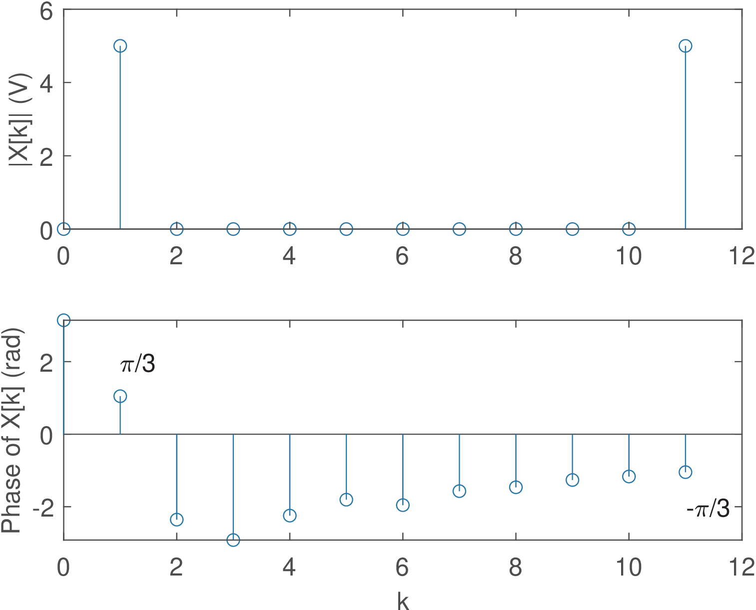
1N=12; %period in samples 
2n=transpose(0:N-1); %column vector representing abscissa 
3Vp=10; x=Vp*cos(pi/6*n + pi/3); %cosine with amplitude 10 V 
4X=(1/N)*fft(x);%calculate DFT and normalize to obtain DTFS 
5A=ak_fftmtx(N,2); %DFT matrix with the DTFS normalization 
6X2=A*x; %calculate the DTFS via the normalized DFT matrix
  

While DFT graphs typically show only the chosen range of $N$ coefficients as in Figure 2.14 and Figure 2.38, sometimes the periodicity of DTFS / DFT must be represented. Therefore, the strict representation of the spectrum of $x[n]$ is given in Figure 2.15, which does not limit the abscissa to $N$ values of $k$.

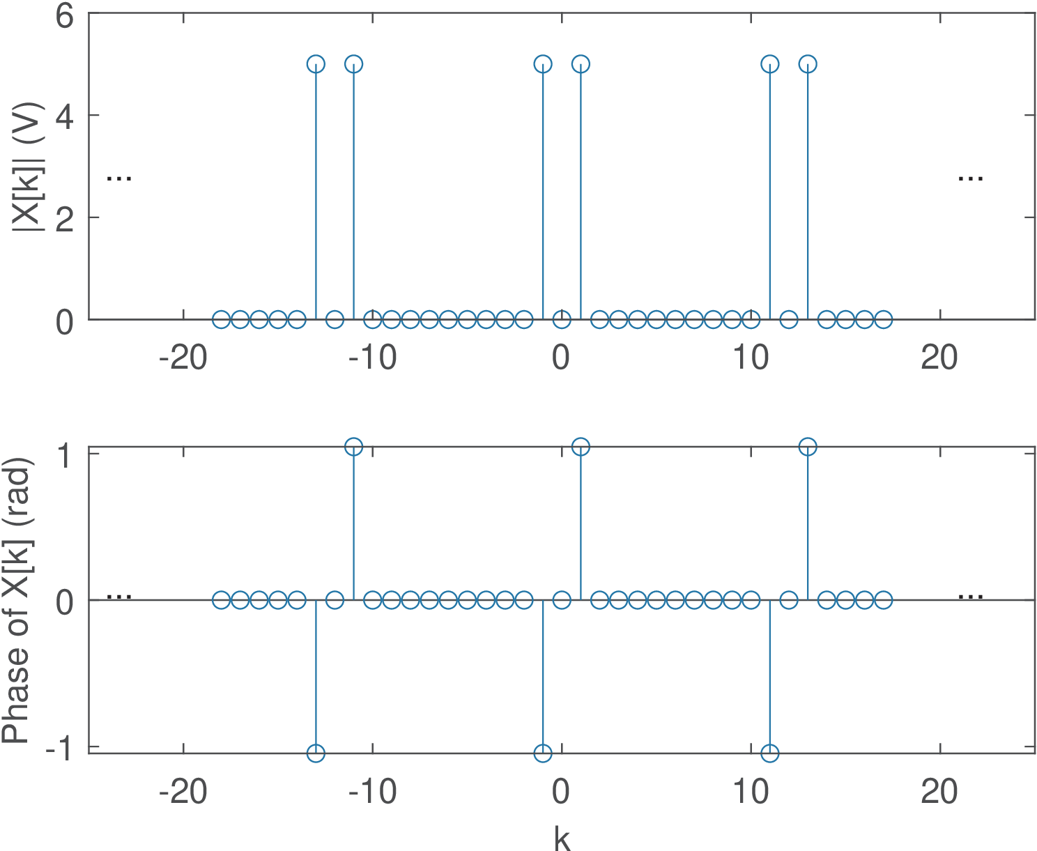
Note in the example of Figure 2.15 the value $N=12$ was chosen to coincide with the period of the cosine and the non-zero coefficients were $k=\pm 1$. Choosing $N=24$ would move the non-zero coefficients to $k=\pm 2$. If the number of points of the DFT / DTFS was not a multiple of 12, $x[n]$ would still be interpreted as a periodic signal but not a single cosine. In this case the spectrum would have many non-zero coefficients.    $\text{□}$

As mentioned, all four pairs of Fourier representations are related. The two pairs of series have been discussed. One can obtain the expressions for transforms from expressions for series by using the limit when the period ($N$ or $T_0$) goes to infinite. This allows to create an aperiodic signal from a periodic one, and also illustrates that the discrete components of the spectrum ($c_k$ or $X[k]$) get so close to each other that create a continuum of frequencies ($X(f)$ or $X(e^{j\mathrm{\Omega }})$). The next sections discuss Fourier transforms.

2.5.3  Continuous-time Fourier transform using frequency in Hertz

The continuous-time Fourier transform¹¹ uses an infinite number of exponentials $e^{\mathit{j\omega t}}$ as basis functions, where $\omega$ is the angular frequency in radians per second and varies from $-\infty$ to $\infty$. Recall from Result 2.1 that two exponentials $e^{j{\omega }_{0}t}$ and $e^{j{\omega }_{1}t}$, ${\omega }_0\ne {\omega }_1$, are orthogonal, and $\omega =2\mathit{\pi f}$, where $f$ is the frequency in Hertz. Hence, the continuous-time Fourier equations are given by

One should interpret the coefficient $X(f_0)$ for a given frequency $f_0$ as the inner product $X(f_0)=⟨x(t),e^{j2\pi f_{0}t}⟩$.

As anticipated in Table 2.5, if $x(t)$ is given in volts, the unit of $X(f)$ is volts $\times$ seconds or, equivalently, volts/Hz. Similarly, for $x(t)$ in ampere, $X(f)$ is in ampere/Hz, and so on.

2.5.4  Continuous-time Fourier transform using frequency in rad/s

In some applications of Fourier transform, it is more convenient to use $X(\omega )$ with $\omega$ in rad/s, instead of $X(f)$ with $f$ in Hz.

Having $X(\omega )$ as a convenient alternative to $X(f)$, where $\omega =2\mathit{\pi f}$, is very different from deriving a new function $Y(f)=X(2\mathit{\pi f})$ by contracting the frequency axis by the factor $2\pi$ (see, e. g., Figure 1.6). In case $Y(f)=X(2\mathit{\pi f})$, the two functions $Y(f)$ and $X(f)$ are different. In contrast, $X(f)$ and $X(\omega )=X(2\mathit{\pi f})$ represent the very same function, but with distinct independent variables. In summary, a plot of $X(f)$ without impulses $\delta (f)$ can be converted to $X(\omega )$ by simply multiplying the abscissa by $2\pi$. But due to the scaling property of the impulse, the area of each eventual impulse in $X(f)$ needs to be scaled by $2\pi$ when representing it in $X(\omega )$. Some examples are provided in the sequel.

Example 2.19. Examples contrasting Fourier transforms in linear and angular frequencies As depicted in Figure 2.16, when there are no impulses in $X(f)$, the Fourier transform $X(\omega )$ is obtained by simply multiplying the abscissa by $2\pi$.

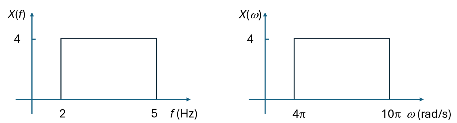
However, when $X(f)$ contains impulses, the scaling property of an impulse described in Appendix A.26.5.0 has to be taken into account. This property states that each area $A$ of an impulse $\mathit{A\delta }(f)$ in $X(f)$ is multiplied by $2\pi$ to become $2\mathit{\pi A\delta }(\omega )$ in $X(\omega )$. For example, the transform of $x(t)=\text{cos}<!--\; FUNCTION\; APPLICATION\; -->(2\pi f_{0}t)$ is $X(f)=0.5[\delta (f+f_0)+\delta (f-f_0)]$ or, equivalently, $X(\omega )=\pi [\delta (\omega +2\pi f_0)+\delta (\omega -2\pi f_0)]$. Figure 2.17 provides an example for $x(t)=6\text{cos}<!--\; FUNCTION\; APPLICATION\; -->(10\mathit{\pi t})$.

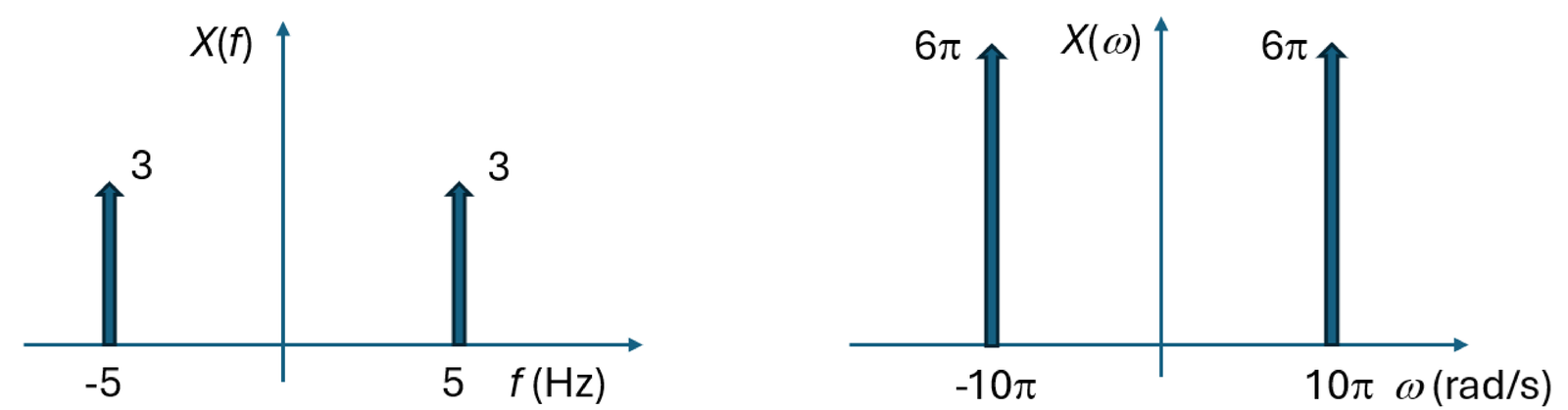
It is instructive to compare Figure 2.16 and Figure 2.17, observing that $X(f)$ and $X(\omega )$ are two distinct representations of the same Fourier transform of the respective signal $x(t)$.

As a final example, consider that $X(f)=5\mathrm{\text{rect}}(f∕4)+3\delta (f-2)$ is the Fourier transform of a complex-valued signal $x(t)$. The spectrum $X(f)$ does not have Hermitian symmetry because $x(t)$ is not real-valued. When $\omega$ in rad/s is adopted, this spectrum is represented as $X(\omega )=5\mathrm{\text{rect}}\left(\omega ∕(8\pi )\right)+6\mathit{\pi \delta }(\omega -4\pi )$. The amplitude of the $\mathrm{\text{rect}}(\cdot )$ function is 5 in both $X(f)$ and $X(\omega )$, but the area of the impulse is scaled by $2\pi$ in $X(\omega )$.    $\text{□}$

Because they represent the same spectrum, $X(f)$ and $X(\omega )$ share the same properties with few subtle differences imposed by the factor $2\pi$. If a given property is defined for one of these two functions (the “mother” definition for this property), an equivalent property can be derived for the other (“child” definition).

For instance, assume the Fourier transform given in Hertz is the “mother” definition described by Eq. (2.31). The “child” definition using rad/s instead of Hz, requires a change of variable $f=\frac{\omega }{2\pi }$ to obtain the alternative Fourier transform definition:

given that $\mathrm{\text{d}}f=\frac{\mathrm{\text{d}}\omega }{2\pi }$.

Units of the Fourier transform in linear and angular frequencies

Table 2.5 indicated that, when $x(t)$ is given in volts, the unit of $X(f)$ is volts/Hz. The unit of $X(\omega )∕(2\pi )$ is volts/(rad/s), and the need to incorporate the $2\pi$ factor is better understood via an example.

For instance, when $X(f)=5\mathrm{\text{rect}}(f∕4)$, the value is 5 V/Hz from $[-2,2]$ Hz, and zero otherwise. The integral of $X(f)$ is 20 volts, because:

Equivalently, this spectrum can be denoted as $X(\omega )=5\mathrm{\text{rect}}(f∕(8\pi ))$. The unit of $X(\omega )$ is not directly in volts/(rad/s) because taking the value of 5 along the frequency band $[-4\pi ,4\pi ]$ leads to

But using a normalization factor of $2\pi$, the function $X(\omega )∕(2\pi )$ can be interpreted in units of rad/s. For the given example, one has a density of $5∕(2\pi )$ V/(rad/s), which leads to

Hence, the factor $\frac{1}{2\pi }$ in Eq. (2.32) is essential for having the proper results and interpreting $X(\omega )∕(2\pi )$ in units of volts/(rad/s). For example, for $t=0$

2.5.5  Discrete-time Fourier transform (DTFT)

The discrete-time Fourier transform uses an infinite number of exponentials $e^{j\mathrm{\Omega }n}$ as basis functions, where $\mathrm{\Omega }$ is the angular frequency in radians. The equations are given by

If $x[n]$ is given in volts, the unit of $X(e^{j\mathrm{\Omega }})∕(2\pi )$ is volts per radians. For instance, assuming $X(e^{j\mathrm{\Omega }})=10\pi \mathrm{\text{rect}}(\mathrm{\Omega })$, the density is $X(e^{j\mathrm{\Omega }})∕(2\pi )=5$ volts/rads over the frequency band $\mathrm{\Omega }\in [-0.5,0.5]$ rads, and one has

One should interpret the coefficient $X({\mathrm{\Omega }}_0)$ for a given frequency ${\mathrm{\Omega }}_0$ as the inner product $X({\mathrm{\Omega }}_0)=⟨x[n],e^{j{\mathrm{\Omega }}_{0}n}⟩$.

The notation is $X(e^{j\mathrm{\Omega }})$ because $\mathrm{\Omega }$ only appears in the imaginary part of an exponent, i. e., $\mathrm{\Omega }$ is always the angle of a complex exponential, unless $\mathrm{\Omega }$ is the argument of an impulse $\delta (\mathrm{\Omega })$. For example, $X(e^{j\mathrm{\Omega }})=\frac{1+\mathrm{\Omega }}{3+\mathrm{\Omega }}$ will never be a “valid” discrete-time Fourier transform for the signals of interest. In contrast, a “valid” expression is $X(e^{j\mathrm{\Omega }})=\frac{1+e^{j2\mathrm{\Omega }}}{3+e^{-j4\mathrm{\Omega }}}+\delta (\mathrm{\Omega })$. One can also note that

which indicates that $X(e^{j\mathrm{\Omega }})$ is always periodic in $2\pi$ (for any $x[n]$). This discreteness-periodicity duality had been already summarized in Table 2.4.

Calculating the DTFT via the DFT

The DFT corresponds to sampling the DTFT in the frequency domain such that

with $N$ being the DFT dimension. In other words, the DFT uses a frequency increment of $\mathrm{\Delta }\mathrm{\Omega }=2\pi ∕N$ and calculates the value of the DTFT $X(e^{j\mathrm{\Omega }})$ at the angles $0,\mathrm{\Delta }\mathrm{\Omega },2\mathrm{\Delta }\mathrm{\Omega },\dots ,(N-1)\mathrm{\Delta }\mathrm{\Omega }$ rad.

The discrete-values of the angles used in an $N$-point DFT are called DFT (or FFT) bins. Hence, in Fourier analysis, the number of bins coincides with the number $N$ of DFT / FFT points. Figure 2.18 depicts an example with $N=4$. In this case, a cosine $x[n]=\text{cos}<!--\; FUNCTION\; APPLICATION\; -->((\pi ∕2)n)$ with angular frequency ${\mathrm{\Omega }}_c=\pi ∕2$ is called bin-centered because its frequency coincides with a DFT bin (also called DFT frequency line).¹²

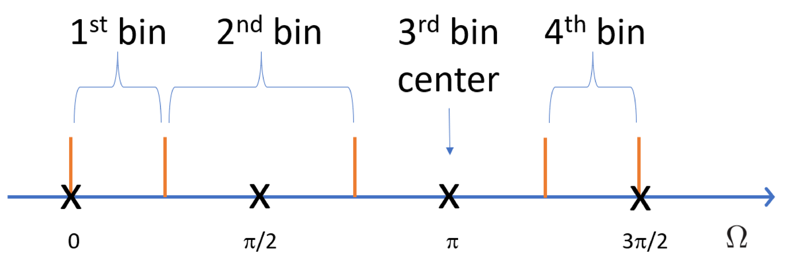
Figure 2.18 has similarities to the histogram in Figure 1.21. For instance, for the DFT one can assume that the minimum and maximum angular frequencies are always $\mathrm{\Omega }=0$ and $2\pi$, respectively. Hence, the bin width can be calculated using a strategy similar to the one adopted in Eq. (1.15), as $\mathrm{\Delta }\mathrm{\Omega }=(2\pi -0)∕N=2\pi ∕N$. However, the bin centers in histograms are calculated differently than DFT bin centers. A histogram with $B$ bins uses the minimum signal value as an edge of the first bin. In contrast, as indicated in Figure 2.18, the minimum angular frequency value $\mathrm{\Omega }=0$ rad is considered to be the first bin center (not the edge). Because of this, the first and last bins of a DFT/FFT have a width of $\mathrm{\Delta }\mathrm{\Omega }∕2$, which differs from the other bins.

Another issue when using a DFT is to improve its resolution given by $\mathrm{\Delta }\mathrm{\Omega }=2\pi ∕N$. When one wants to sample the DTFT using a high-resolution grid, the value $N$ is chosen to be larger than the duration of $x[n]$ and zero-padding is adopted. Zero-padding corresponds to simply increasing the size of a sequence by appending extra values to it, all with zero amplitude.