Exercises

2.13 Exercises

2.1. A segment of an ECG signal $x [n]$ with six samples $[- 1, 0.6, 0.5, 1, 2.5, 2]$ must be encoded using a 3-points DCT (i. e., using two frames with three samples each). Find the DCT coefficients of these two vectors. Then, reconstruct an approximation of the two vectors assuming that only the first coefficient can be used while the other two are discarded (assumed to be zero). Confirm Eq. (2.24) calculating the norms of both error vectors $e_{t}$ and $e_{f}$ .
2.2. A segment of an ECG signal with four samples $[0.5, 1, 2.5, 2]$ must be encoded using a 2-points DCT (i. e., using two frames with two samples each). The coefficients at the DCT domain must be quantized with 4 bits per frame, with the first coefficient (DC) being quantized with 3 bits and the other one with 1 bit. Both quantizers have a step of $Δ = 0.5$ and their first output level is $0.25$ . a) What is the decoded signal (after coding and decoding)? b) What is the mean squared-error? c) What is the SNR in dB? d) What is the bit rate in bps assuming $F_{s} = 150$ Hz? e) What is the bit rate and SNR if the second coefficient is discarded (no bits are allocated for it and its value is assumed to be zero during decoding)?
2.3. Consider that a block of pixels $C = [\begin{matrix} 120 & 140 & 139 \\ 124 & 220 & 120 \\ 114 & 130 & 122 \end{matrix}]$ was extracted from an image. Calculate the bi-dimensional DCT and DFT first processing each row and organizing the result of this intermediate step as a matrix $T$ , then apply the transforms to each column of $T$ to generate the final matrix. Follow this procedure to obtain a matrix with the DCT coefficients and then repeat it to obtain the DFT coefficients.
2.4. Design a DCT-based image coding system that is capable of handling 24 bits/pixel color images and 8 bits/pixel black and white (B&W, also called gray) images, all with a size of 512 $\times$ 512 pixels. The system should operate using: a) 3 bits/pixel, b) 1 bit/pixel or c) 0.25 bit/pixel. For the three cases, provide the average peak SNR (PSNR), i. e., the SNR when assuming the “signal” in the numerator is an image with all pixels at the peak value of 255 and the denominator is the mean squared-error. The test sequence should be the colorful and B&W versions of the images Lenna, Peppers, Baboon, Splash and Tiffany, available from [ url2us2]. Do not download B&W versions of the five mentioned images, but make the conversion from color to B&W yourself and describe the conversion method you used. Hence, the test set will have 5 images. You can use as many images you want to compose your training set (distinct from the test set images). Provide the source code and a short report of your results that includes the average PSNR.
2.5. Use the Gram-Schmidt procedure to find an orthonormal basis to represent the vectors in the set $C = {[0, 0, 1], [0, 1, 0], [0, 0, 8], [0, 5, 0], [4, 1, 2], [0, 0, 3]}$ . Show also that any vector in $C$ can be written as a linear combination of the obtained basis vectors.
2.6. KLT (or PCA) is the optimal linear transform for coding. But one needs to remember that PCA assumes the signal is zero mean. This exercise uses this fact to exemplify the importance of following the assumed model (in this case, that the signal is zero mean). Design a coding system for the data x below.

Listing 2.13: MatlabOctaveCodeSnippets/snip_transforms_KLT.m. [ Python version]

1N=100; %number of vectors 
2K=4;   %vector dimension 
3line=1:N*K; %straight line 
4noisePower=2; %noise power in Watts 
5temp=transpose(reshape(line,K,N)); %block signal 
6x=temp + sqrt(noisePower) * randn(size(temp)); %add (AWGN) noise 
7z=transpose(x); plot(z(:)) %prepare for plot

Because PCA / KLT does not model the mean, in practice, one needs to extract the mean from the data and later recover it for final reconstruction. And, eventually, one also normalizes the variances to be equal to one. This normalization is called in statistics to “z-transform” the data, but this term should not be confused with the Z transform.
2.7. Generate $N = 10, 000$ samples from a bidimensional Gaussian $f_{X_{1}, X_{2}} (x_{1}, x_{2})$ with mean $\hat{μ} = {(30, - 20)}^{T}$ and covariance matrix $C = [\begin{matrix} 10 & 0.99 \\ 0.99 & 40 \end{matrix}]$ . Obtain two transforms: $A_{g}$ using Gram-Schmidt orthonormalization and $A_{p}$ using PCA. You can remove means if useful. Using each transform, project the data into the new space and compute the variance of the coefficients in each dimension. Which transform you expect to lead to smaller variances of the transformed vectors?
2.8. Following a scheme similar to the one presented in Application 2.4 - ECG Coding, compare the performance of KLT and DCT using a test set of at least 50 ECT records from the MIT-BIH Arrhythmia Database. Note that for performing any preparation / training you should use a training set, disjoint of the test set. Otherwise your results can be biased by the fact that you already knew what should be coded.
2.9. Calculate “manually” the DFT of the sequence $x [n] = [2, 0, 2, 0]$ . Then use the fft function in Matlab/Octave and compare the results.
2.10. What are the forward $A$ and inverse $A^{H}$ matrices for a 3-points orthonormal DFT?
2.11. Consider that $s [n]$ was obtained by sampling with $F_{s} = 100$ kHz an analog and periodic signal $s (t)$ . The sampling theorem was obeyed. The 8-DFT of $s [n]$ was calculated in Matlab/Octave with fft(s)/N and is shown in Figure 2.49. The value $N$ was chosen to be an exact multiple of the fundamental period of $s (t)$ such that the problem of spurious components illustrated in Figure 2.42 did not occur. a) What is the frequency of each component of $s (t)$ ? b) What is the resolution $Δ f$ in Hz of this DFT? c) Find a reasonable expression for $s (t)$ .

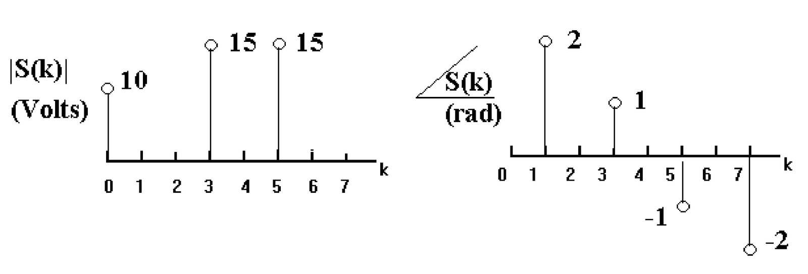
Figure 2.49: DFT with $N = 8$ points of a signal sampled at $F_{s} = 100$ kHz.

2.12. Given that

X = [8, 0, 0, 0]

was obtained with a 4-points orthonormal DFT, find its inverse

x

. For the same spectrum, assuming that

F_{s} = 10

Hz, to which frequencies correspond the elements of

X

?
2.13. Consider that a periodic

x (t)

was sampled with

F_{s} = 20

Hz, obeying the sampling theorem. A 128-points FFT was calculated using Matlab/Octave and the output

X

was normalized by

N = 128

. The only non-zero coefficients were

k = 0, 3

and 125, corresponding to the elements of

X [1] = 12

X [4] = 3 + j 4

and

X [126] = 3 - j 4

, respectively. a) What is the frequency in Hz of the component with largest power of

x (t)

? b) what is the average (DC) value of

x (t)

? c) what is the spacing in Hz between neighboring elements of

X

? d) what is the maximum frequency found in

x (t)

?
2.14. Using the orthogonality condition of the basis functions derive the pair of Fourier series equations. To do that, recall how the inner product between complex signals is defined using the conjugate, and the normalization factor because the basis are not orthonormal.
2.15. What are the Fourier series coefficients for the signal

x (t) = 2 + 3 cos (2 π 100 t) + 8 sin (2 π 300 t + π) + cos (2 π 50 t - π)

?
2.16. The bilateral Fourier series of a signal

x (t)

with period

T_{0} = 0.01

s has non-zero coefficients

c_{0} = 3

c_{1} = 2 e^{- j 4}

c_{4} = 5

c_{- 1} = 2 e^{j 4}

and

c_{- 4} = 5

. What is the expression for

x (t)

?
2.17. What is the Fourier transform of: a)

x (t) = rect (t)

, b)

y (t) = 4 rect (t - 6)

and c)

z (t) = 5 rect ((t - 4) ∕ 3)

?
2.18. What is the Fourier transform of: a)

x (t) = sinc (t)

, b)

y (t) = 4 sinc (t - 6)

and c)

z (t) = 5 sinc ((t - 4) ∕ 3)

?
2.19. Prove the expressions: a) for the DTFT of

x [n] = 0 . 9^{n} u [n] + 0 . 8^{n} u [n]

and b) for its Z transform, indicating the ROC.
2.20. Considering the range

Ω \in [- π, π [

, the DTFT

H (e^{j Ω})

of a signal is 1 when

- Ω_{c} \leq Ω \leq Ω_{c}

and 0 otherwise (i. e., an ideal low-pass filter). Find its inverse DTFT

h [n]

indicating all steps in this proof.
2.21. Prove that

X (e^{j Ω}) = \sum_{k = - \infty}^{\infty} 2 πδ (Ω - Ω_{0} + 2 πk)

is the DTFT of

x [n] = e^{j Ω_{0} n}

and indicate when the impulse sifting property is used. Using the result, carefully draw the graph of the real part of the DTFT of

y [n] = 3 + 4 e^{jπn}

for the range

- 3 π \leq Ω \leq 3 π

.
2.22. Prove the cited properties of the Fourier tools for the case of the Fourier transform.
2.23. Prove the cited Fourier pairs for the case of the DTFT.
2.24. A right-sided signal has Laplace transform

X (s) = 5 ∕ (s^{2} + 2 s + 10)

, with ROC

σ > - 1

. Calculate: a)

X (s) |_{s = 2}

, b) the corresponding Fourier transform

X (ω)

if it exists and c) if

X (ω)

exists,

| X (ω) |

for

ω = 3

rad/s.
2.25. A signal

x (t)

has Laplace transform

X (s) = (3 s + 2) ∕ ((s - 1) (s - 3))

, with ROC

σ < 1

. Find

x (t)

.
2.26. A signal

x [n]

has Z transform

X (z) = (5 z^{2} + 4 z + 3) ∕ ((z - 0.7) (z - 0.8))

, with ROC

| z | > 0.8

. Find

x [n]

.
2.27. Find the Z transform and associated ROC of the signal

x [n] = - 3^{n} u [- n - 1]

. Does this signal have a DTFT?
2.28. What is the Z transform

X (z)

of the signal

x [n] = 4 δ [n] + 5 δ [n - 11]

? What are the values of

X (z)

for

z = 0, - 1

and

z = 8 e^{jπ}

? If the DTFT of

x [n]

exists, what are its values for

Ω = 0, π

and

2 π

rad?