2.9  Z Transform

The Z transform is the counterpart of the Laplace transform for discrete-time signals. The pair of equations is given by

where $C$ is a counterclockwise closed path encircling the origin and entirely in the region of convergence (ROC). The contour (or path) $C$ must encircle all of the poles of $X(z)$.

2.9.1  Relation between Laplace and Z transforms

The Laplace and Z transforms are related. When the Laplace transform is performed on a sampled signal $x_s(t)$ and a C/D is used, the result is the Z transform¹⁵ of a discrete-time sequence $x[n]$ where

and $T_s$ is the sampling period.

Eq. (2.59) is used in the matched Z-transform method for converting $H(s)$ in $s$ into $H(z)$ in $z$, and is further discussed in Section 3.11.3.

Example 2.23. Converting $x(t)$ to discrete-time and finding the corresponding Z-transform. As in Example 1.33, assume a continuous-time signal $x(t)=4e^{-2t}u(t)$ should be transformed to a discrete-time $x[n]$ with a sampling period $T_s$, and then have its Z-transform $X(z)=Z\{x[n]\}$ calculated. From Eq. (1.34):

where the last step used Eq. (2.61).   $\text{□}$

2.9.2  Advanced: Z transform basis functions

The basis functions of the Z transform are $z^n$, $z\in ℂ$. The complex-value $z$ could be written in Cartesian coordinates but it is more convenient to write it in polar coordinates, as $z=r{e}^{j\mathrm{\Omega }}$. Taking in account the discrete-time $n$, a Z basis function can be written as

Similar to the Laplace basis function $e^{(-\sigma +\mathit{j\omega })t}$, which has $\sigma$ and $\omega$, the Z basis function is also controlled by two parameters: $r$ and $\mathrm{\Omega }$. As $\sigma$ in the Laplace transform, the value of $r$ imposes the envelope of the Z basis function while $\mathrm{\Omega }$ (similar to $\omega$) controls the rate of its oscillation (see Figure 2.20).

The similarity of Laplace and Z basis functions can be made more explicit by writing

where $r=e^{-\sigma }$. Comparing the Laplace basis function $x(t)$ with the Z basis function $x[n]$, it is clear that they describe the same category of signals, but in continuous-time and discrete-time, respectively.

But the region of convergence of a Laplace transform depends on $\sigma$, so it is convenient to write the complex value $s=\sigma +\mathit{j\omega }$ in Cartesian coordinates, to make $\sigma$ explicit. On the other hand, as will be discussed in this section, the region of convergence of a Z transform is determined by the magnitude $r$ of a $z$ value, which makes more convenient to write the complex value $z=r{e}^{j\mathrm{\Omega }}$ in polar coordinates, making $r$ explicit.

2.9.3  Some pairs and properties of the Z-transform

A very useful Z transform pair is

• $\delta [n]\iff 1$

and an important Z transform property is

• $x[n-n_0]\iff X(z)z^{-n_0}$.

Putting them together leads to

• $\delta [n-n_0]\iff z^{-n_0}$.

With this result, and using linearity one can write, e. g.,

In cases $x[n]$ is left-sided or right-sided, $X(z)={\sum <!--\; FUNCTION\; APPLICATION\; -->}_{n=-\infty }^{\infty }x[n]z^{-n}$ can be written as a geometric series and Eq. (A.20) used to obtain $X(z)$. For example, the Z transform of $x[n]=a^{n}u[n]$ is obtained as follows:

Using Eq. (A.20) with a scale factor $\alpha =1$, ratio $r=a{z}^{-1}$ and $|a∕z|<1$ leads to

2.9.4  Region of convergence for a Z transform

Similar to the Laplace transform, the values of $z$ for which the transform exists are called the region of convergence (ROC). The ROC of Z transforms are annular regions of the form $|z|>m$ (for right-sided sequences, also called causal), $|z|<m$ (for left-sided sequences) or $m<|z|<p$ (for two-sided sequences), where $m,p\in {ℝ}_{+}$. When the signal in time-domain has a finite support (duration), the ROC of the associated Z transform is the whole $z$-plane, eventually with the exceptions of $z=0$ and $z=\infty$.

To recover $x[n]$ from its transform $X(z)$, it is essential to know the ROC. For example, the Z transform of $x[n]=-a^{n}u[-n-1]$ is:

In order to use Eq. (A.20) with factor $\alpha =1$ and ratio $r=z∕a$ one can modify the summation interval

with the ROC $|z|<|a|$ (because Eq. (A.20) requires $|z∕a|<1$). In summary, both $a^{n}u[n]$ (see Eq. (2.61)) and $-a^{n}u[-n-1]$ have $X(z)=z∕(z-a)$ and only the ROC can disambiguate them when calculating the inverse Z transform.

2.9.5  Inverse Z of rational functions via partial fractions

In general, the inverse Z transform is calculated using Eq. (2.58). But similar to the methodology described for the Laplace transform in Section 2.8.5, for the important category of Z transforms $X(z)$ that are ratios $X(z)=B(z)∕A(z)$ of two polynomials, one can use partial fraction expansion (see Appendix A.10) to conveniently calculate the inverse $x[n]=Z^{-1}\{X(z)\}$.

The inverse transform of rational functions $X(z)$ can be obtained by following two simple steps and then the procedure in Section 2.8.5 adopted for inverse Laplace transforms. The procedure is the following:

f 1.

make the rational function $X(z)$ to have only non-negative¹⁶ powers of $z$,

f 2.

find the poles and expand $X(z)$ in partial fractions as discussed in Section A.10,

f 3.

eventually multiply by $z$ to create $Y(z)=\mathit{zX}(z)$ and force the appearance of terms term $z∕(z-a)$,

f 4.

convert each parcel of $Y(z)$ to the time domain,

f 5.

rearrange the terms, especially the ones corresponding to complex conjugate poles and

f 6.

because $Y(z)=\mathit{zX}(z)$, then $x[n]=y[n-1]$. Find the final result substituting $n$ by $n-1$ in $y[n]$.

For example, to obtain the inverse transform of

with ROC $|z|>0.8$, one can multiply numerator and denominator by $z^3$ and obtain their roots:

The partial fraction expansion is

Multiplying both sides by $z$ leads to

which can be rewritten by converting the complex numbers from Cartesian to polar form

Because in this case the ROC is for a right-sided sequence, each term $z∕(z-a)$ corresponds to $a^{n}u[n]$ and the time domain signal is

which leads to

Note that a pair of complex conjugate poles have complex conjugate residues. Let $r=b{e}^{\mathit{j\alpha }}$ and $r^{\ast }=b{e}^{-\mathit{j\alpha }}$ be the residues for poles $p=a{e}^{\mathit{j𝜃}}$ and $p^{\ast }=a{e}^{-\mathit{j𝜃}}$, respectively, both with multiplicity one. With a ROC corresponding to right-sided signals, the two terms $\mathit{rz}∕(z-p)$ and $r^{\ast }z∕(z-p^{\ast })$ in the partial fraction expansion can be rearranged in time domain to compose the general expression

If the ROC corresponds to left-sided signals, the same terms correspond to

Different approaches to obtain $x[n]$ can lead to distinct expressions, but these expressions must correspond to the same values of $x[n],\forall <!--\; FUNCTION\; APPLICATION\; -->n$. For example, some people prefer to obtain the partial fraction expansion of $X(z)∕z$ instead of using the suggested steps 3) and 6). Expanding $X(z)∕z$ allows to multiply the obtained partial fractions by $z$ to get $z∕(z-a)$ factors. An example better illustrates the equivalence of both procedures and the reason for suggesting ours.

Assume the task is to find the inverse $x[n]$ of $X(z)=(8z-19)∕[(z-2)(z-3)]$ knowing that $x[n]$ is right-sided. Using the alternative procedure of expanding $X(z)∕z$, one has

which can be conveniently multiplied by $z$ to obtain parcels in the form $z∕(z-a)$:

that leads to the inverse

Using the steps of the suggested procedure, which expands $X(z)$ in partial fractions instead of $X(z)∕z$, the result is

which seems different than Eq. (2.62). However, a closer inspection indicates that, for both expressions, the sample values $x[0]=0,x[1]=8$, etc., are the same, i. e., the procedures led to the same signal, as expected.

Simplifying the partial fractions corresponding to complex conjugates

The Web has several tables of properties and pairs related to the Z transform.¹⁷ An interesting result is the initial value theorem, which is valid for signals for which $x[n]=0$ for $n<0$ (right-sided) and states that

Using this theorem, one can anticipate that $x[0]=0$ when $X(z)$ has a denominator with degree larger than the numerator, such as in $X(z)=(8z-19)∕[(z-2)(z-3)]$.

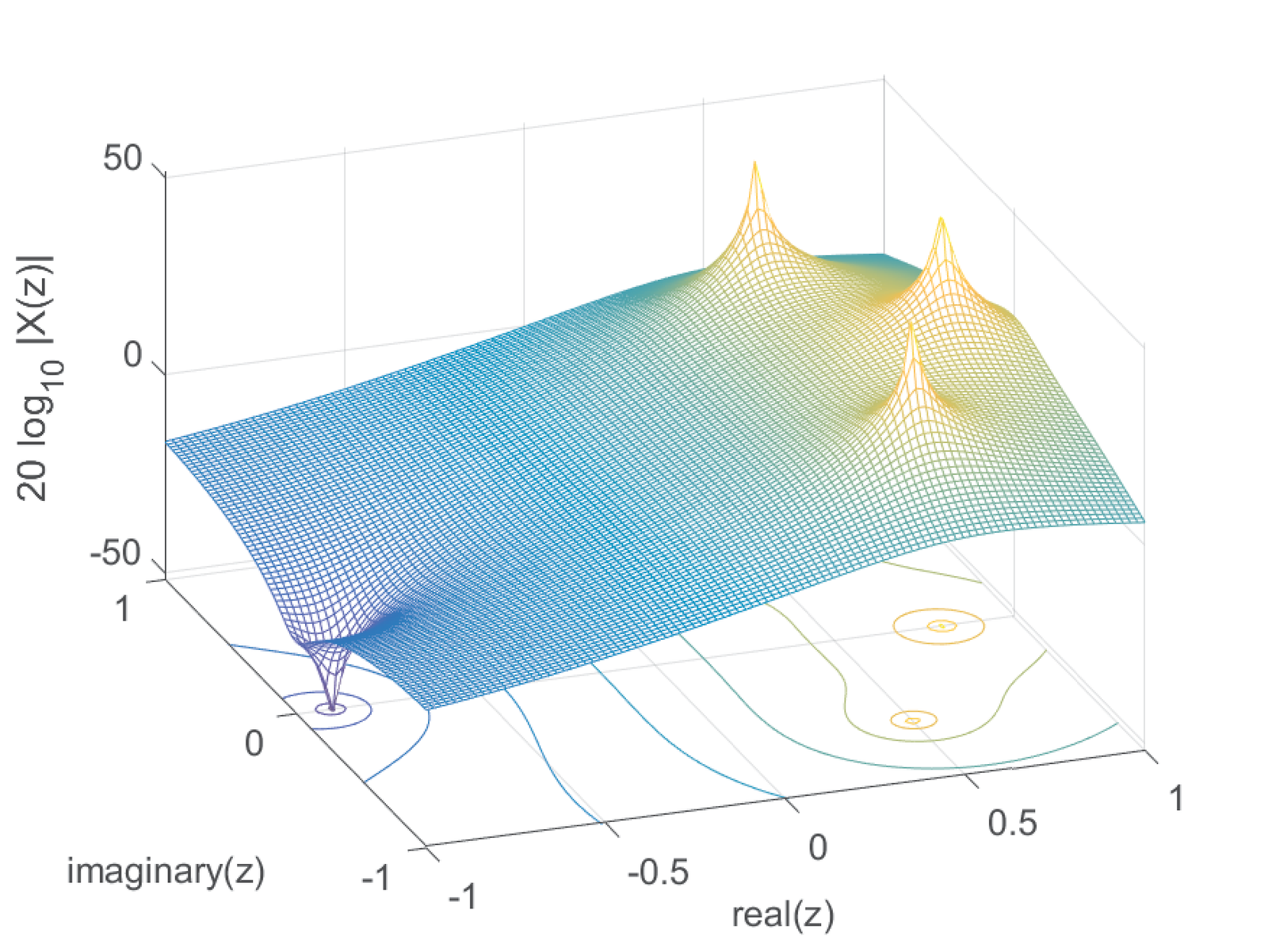
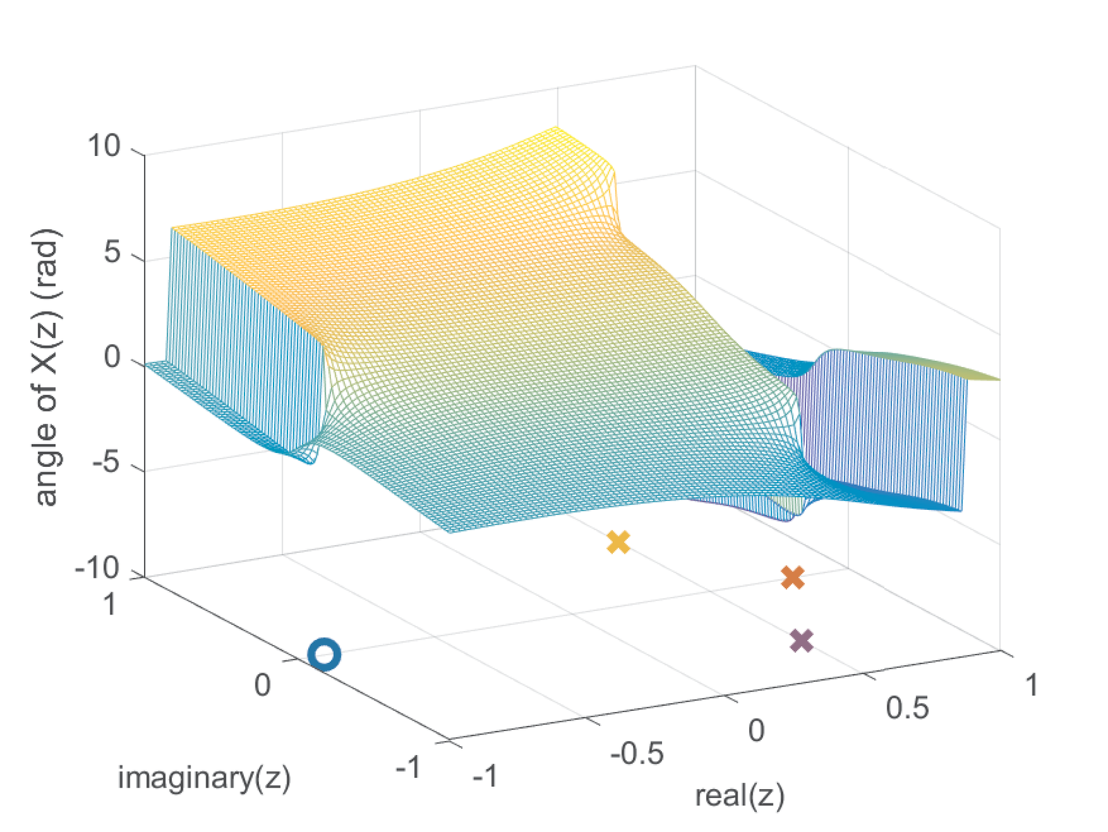
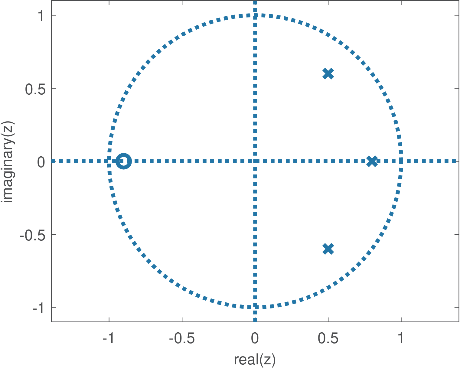
Similar to Figure 2.22 and Figure 2.23, which are for Laplace, Figure 2.27 and Figure 2.28 depicts the magnitude and phase, respectively, for

which has one finite zero and three poles as indicated in Figure 2.29.

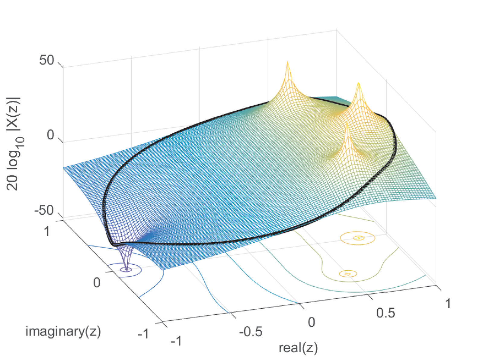
2.9.6  Calculating the DTFT from a Z transform

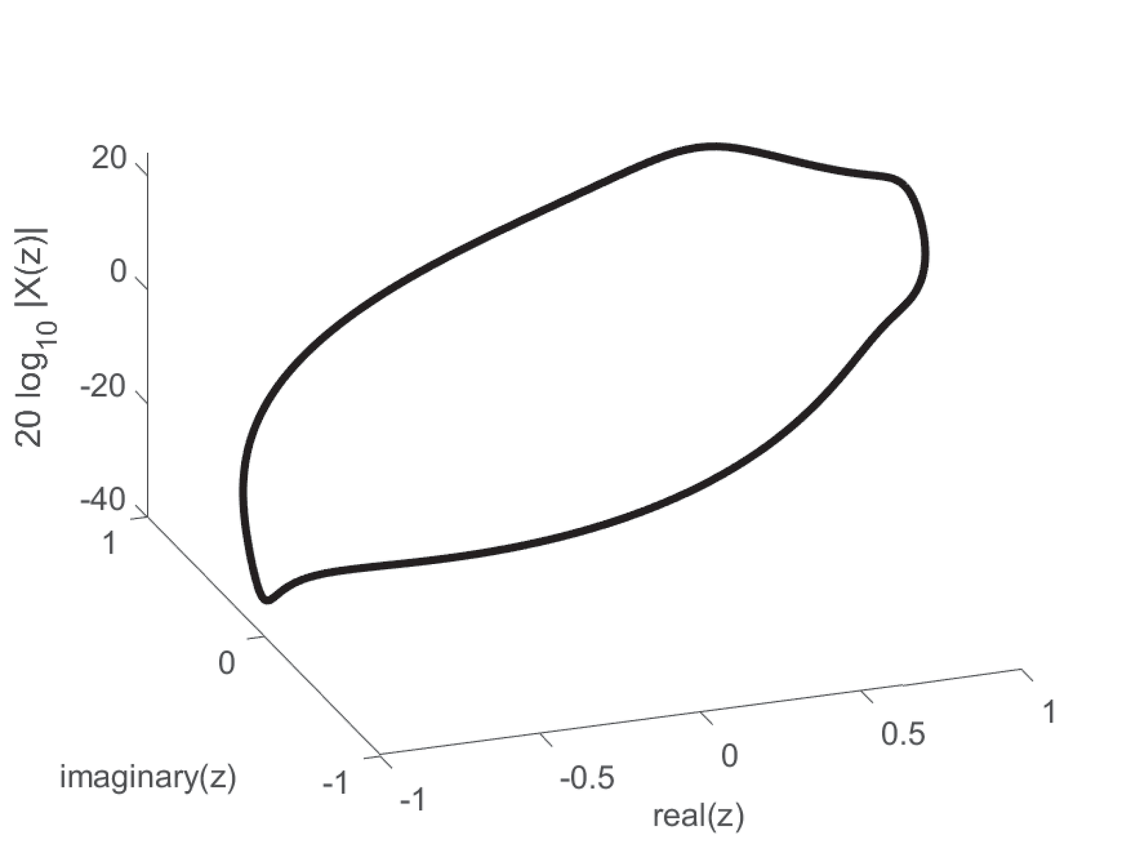
The relation between the Z transform and the DTFT is similar to the one between Laplace and Fourier transforms discussed in Section 2.8.6. Figure 2.30 and Figure 2.31 provide an example using Eq. (2.63).

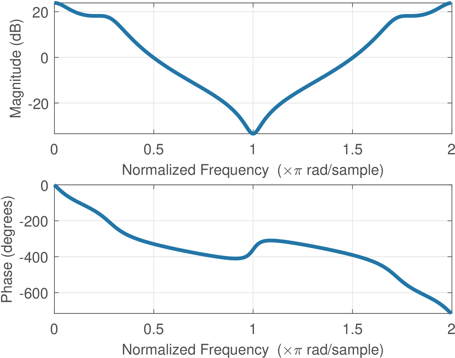
Sometimes it is not convenient to deal with 3-d plots such as Figure 2.31. An alternative is to represent the DTFT using a figure similar to Figure 2.32, which shows the magnitude and phase with the angle as independent variable. As discussed in Section 1.8.4, for convenience, the abscissa is normalized by $\pi$, such that “1” corresponds to $\pi$ rad. Due to the symmetry of $X(z)$ when $x[n]$ is real, it is also common to represent the abscissa in the range $[0,\pi ]$ (instead of $[0,2\pi [$ as in Figure 2.32).