2.8  Laplace Transform

We start our study of Laplace transform by motivating it as an extension of the Fourier transform.

2.8.1  Motivation to the Laplace transform

The Fourier analysis is not able to provide a representation for some specific signals. For example, the signal $x(t)=e^{3t}u(t)$, does not have a Fourier transform because the integral

does not converge. Note that one should evaluate

considering that $|e^{\mathit{j\omega t}}|=1$ (this limit is not $\infty ∕\infty$ and L’Hospital’s rule is not appropriate).

This limitation in the representational power of Fourier analysis can be circumvented with the trick of pre-multiplying the input signal by an exponential. Assuming the continuous-time domain, this corresponds to multiplying $x(t)$ by an exponential $e^{-\mathit{\sigma t}}$, $\sigma \in ℝ$, and then taking the Fourier transform of $x(t)e^{-\mathit{\sigma t}}$. For example, if $x(t)=e^{3t}u(t)$, then pre-multiplying by $e^{-4t}$ leads to the following Fourier transform for $z(t)=x(t)e^{-4t}=e^{-t}u(t)$:

The signal $x(t)$ could be recovered from the inverse Fourier transform of $Z(\sigma ,\omega )$ and a post-multiplication by $e^{4t}$. This trick can be adopted with several different values of $\sigma$. For example, $z(t)=x(t)e^{-5t}$ would also work in the previous example, as well as all values of $\sigma$ such that $\sigma >3$ (note that the exponent of $e^{-\mathit{\sigma t}}$ uses $-\sigma$, not $\sigma$).

Based on this motivation, the Laplace transform $X(s)$, where $s=\sigma +\mathit{j\omega }$ is a complex number, can be interpreted as the Fourier transform of the signal multiplied by the exponential $e^{-\mathit{\sigma t}}$, as follows:

The pair of Laplace equations is defined as:

where $\gamma$ is a real number so that the contour path of integration is in the region of convergence of $X(s)$. Because there are two parameters, $\sigma$ and $\omega$, the values that $s=\sigma +\mathit{j\omega }$ can assume as the independent variable of a Laplace transform $X(s)$ compose a plane, while in the Fourier transform $X(\omega )$ the independent variable the angular frequency $\omega$ (the abscissa line, not a plane).

As will be discussed in Chapter 3, the choice of $e^{\mathit{st}}$ and the corresponding popularity of the Laplace transform is due to their use as a tool for analyzing systems not signals.

2.8.2  Advanced: Laplace transform basis functions

One can interpret the Laplace transform as having basis functions $e^{(-\sigma +\mathit{j\omega })t}$ with two parameters $\sigma$ and $\omega$. The Laplace transform can then be seen as obtaining coefficients from inner products $⟨x(t),e^{(-\sigma +\mathit{j\omega })t}⟩$, given that the complex conjugate of the basis function is $e^{(-\sigma -\mathit{j\omega })t}=e^{-\mathit{st}}$.

But an interesting distinction between the Fourier and Laplace transforms is the following. When using the Fourier transform, if the signal coincides with a given basis function (e. g., $x(t)=\text{cos}<!--\; FUNCTION\; APPLICATION\; -->({\omega }_{0}t)$), a signal impulse represents the signal in the transform domain ($X(\omega )=\mathit{\pi \delta }(\omega -{\omega }_0)$ for the given example). This impulse indicates that a single basis functions represents the input signal $x(t)$. Such situations do not occur when the Laplace transform is used. The transform domain $X(s)$ does not use impulses and there is no signal $x(t)$ that is represented by a single basis function.

It is intuitive that the Fourier basis functions, which are limited in amplitude, are not the most adequate to represent a signal such as the $x(t)=e^{3t}u(t)$, which has magnitude increasing with $t$ for $t>0$. Consider picking a very large value $X(f\prime )$ for the Fourier “coefficient” corresponding to the basis function $e^{j2\mathit{\pi f}\mathit{\prime t}}=\text{cos}<!--\; FUNCTION\; APPLICATION\; -->(2\mathit{\pi f}\mathit{\prime t})+j\text{sin}<!--\; FUNCTION\; APPLICATION\; -->(2\mathit{\pi f}\mathit{\prime t})$, this value $X(f\prime )$ would scale the basis along all the time axis, eventually failing to provide a sharp increase in magnitude because $\text{sin}<!--\; FUNCTION\; APPLICATION\; -->(\cdot )$ and $\text{cos}<!--\; FUNCTION\; APPLICATION\; -->(\cdot )$ have amplitudes limited to the range $[-1,1]$.

As mentioned, the Laplace transform multiplies $x(t)$ by an exponential weighting function $e^{-\mathit{\sigma t}}$, where $\sigma \in ℝ$ can control the amplitude of the exponential, which increases and decreases with $t$ for $\sigma <0$ and $\sigma >0$, respectively. By multiplying the exponential sinusoid $e^{\mathit{j\omega t}}$ by $e^{-\mathit{\sigma t}}$, the new basis function $e^{(-\sigma +\mathit{j\omega })t}$ can represent a broader variety of signals.

As an example, the left graph in Figure 2.20 was obtained with Listing 2.3 and the second graph used $\sigma =0.3$ ($\sigma$ is denoted in the code as sigma), with both showing the real part of $e^{(-\sigma +\mathit{j\omega })t}$, with $s=\pm 0.3+j10\pi$. The envelope $e^{\pm 0.3t}$ imposes the peak amplitude of the sinusoid $e^{j10\mathit{\pi t}}$ of 5 Hz.

1sigma = -0.3; w = 2*pi*5; %frequency of 5 Hz 
2z=-sigma+1j*w; %define a complex variable z 
3t=linspace(0,3,1000); %interval from [0, 3] sec. 
4x=exp(z*t); %the Laplace basis function 
5envelope = exp(-sigma*t); %the signal envelope 
6subplot(121);plot(t,real(x));hold on,plot(t,envelope,':r')
  

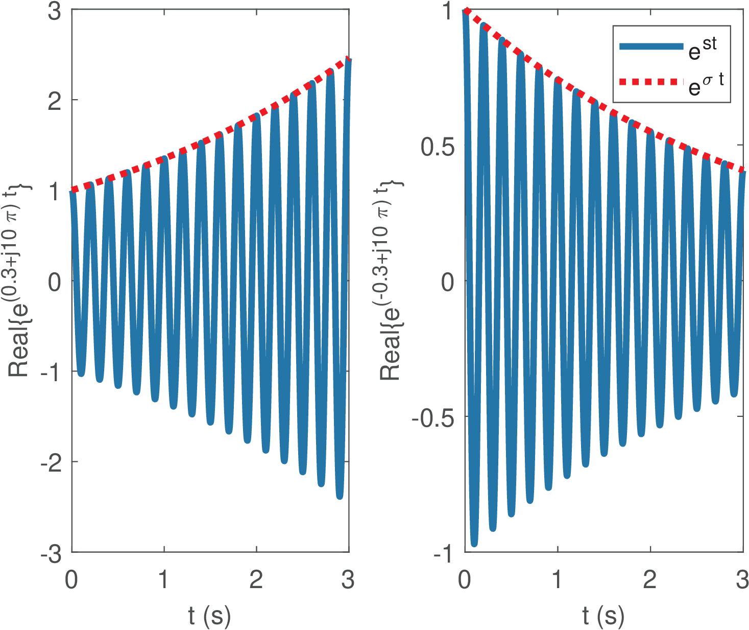
The basis functions $e^{(-\sigma +\mathit{j\omega })t}$ have some peculiarities. If $\sigma <0$ their amplitudes reach $\infty$ when $t\to \infty$. If $\sigma >0$ their amplitudes reach $\infty$ when $t\to -\infty$. Therefore, the Laplace transform is more useful in the analysis of one-sided signals, such as the ones that incorporate $u(t)$ (right-sided, also called causal) or $u(-t)$ (left-sided or anti-causal). In these cases, the basis function do not create mathematical problems at infinite because the ROC is chosen in a way that the signal itself is zero at the problematic limiting values $t=\infty$ or $-\infty$.

2.8.3  Laplace transform of one-sided exponentials

Using Eq. (2.50) and assuming a complex-valued $a\in ℂ$, it is useful to calculate and get familiar with the Laplace transform for the causal $x(t)=e^{\mathit{at}}u(t)$ and anti-causal $x(t)=-e^{\mathit{at}}u(-t)$ signals. Before discussing ROCs in general, it is useful to study the ROCs and transform pairs of these two signals:

and

These pairs are widely proved and discussed in the literature (see, e. g. [ url2roc]). The next example proves Eq. (2.52).

Example 2.20. A time-domain complex exponential leads to a rational function in $s$. Consider $a\in ℂ$ and the following Laplace transform pair

This result is proved as follows:

Given that $s=\sigma +\mathit{j\omega }$, the limit can be obtained as

when $R\mathit{eal}\{a-\sigma \}<0$ (note $|e^{\mathit{j\omega t}}|=1$ and only the numerator defines the convergence).   $\text{□}$

Knowing $X(s)$ does not suffice to uniquely identify $x(t)$, because the two different signals $x(t)$ have the same Laplace transform $X(s)=1∕(s-a)$. Hence, the information about the values of $R\mathit{eal}\{s\}=\sigma$ for which the Fourier transform in Eq. (2.50) converges, must be known too in order to properly identify the original $x(t)$ when recovering it from $X(s)$. In summary, distinct signals $x(t)$ can have the same $X(s)$, differing only in their regions of convergence. This fact will be further explored in the next subsections.

2.8.4  Region of convergence for a Laplace transform

The values of $s$ for which the associated Fourier transform $F\{x(t)e^{-\mathit{\sigma t}}\}$ converges compose the so-called region of convergence (ROC) of the Laplace transform. Observing Eq. (2.52) and Eq. (2.53), one can conclude that for these signals, the ROC is a region $\sigma <a$ at the left of $a$ or at the right ($\sigma >a$).

This can be generalized and, in fact, the ROC of Laplace transforms are always defined by ranges that depend solely on $\sigma$ (the angular frequency $\omega$ does not influence ROCs). For any signal $x(t)$, the Laplace transform convergence depends on $\sigma$, and the ROCs are regions formed at the left or right of a given value ${\sigma }_0$. When $x(t)$ is right-sided, the ROC is the area at the right of some ${\sigma }_0$, while for left-sided $x(t)$ the ROC is the area at the left of a value ${\sigma }_0$. When $x(t)$ is composed by several parcel, the ROC is the intersection of the ROCs of these parcels.

For instance, $y(t)=e^{-3t}u(t)$ has Laplace transform $Y(s)=1∕(s+3)$ with ROC $\sigma >-3$. The anti-causal signal $z(t)=-e^{2t}u(-t)$ has Laplace transform $Z(s)=1∕(s-2)$ with ROC $\sigma <2$. Because the Laplace is a linear transform, the bilateral signal $x(t)=y(t)+z(t)$ has Laplace transform $X(s)=Y(s)+Z(s)$ with the ROC being $-3<\sigma <2$, the intersection between the ROCs of $Y(s)$ and $Z(s)$.

Another example that $x(t)$ can be recovered from the knowledge of $X(s)$ and its associated ROC is the following.

Example 2.21. Distinct signals may have the same Laplace transform, and only the ROC can disambiguate. Given the Laplace transform $X(s)=1∕(s+2)$, one should find the corresponding signal $x(t)$. In fact, there are two possible signals, depending on the ROC. The pole is at $s=-2$ and assuming the ROC is $R\mathit{eal}\{s\}>-2$, then $x(t)=e^{-2t}u(t)$. If the ROC is $R\mathit{eal}\{s\}<-2$, then $x(t)=-e^{-2t}u(-t)$.   $\text{□}$

2.8.5  Inverse Laplace of rational functions via partial fractions

In general, the inverse Laplace transform is calculated using Eq. (2.51). But for the specific, and very important category of Laplace transforms $X(s)$ that are ratios $X(s)=B(s)∕A(s)$ of two polynomials, one can use partial fraction expansion (see Appendix A.10) to conveniently calculate the inverse $x(t)=L^{-1}\{X(s)\}$.

The inverse transform of a rational function $X(s)=B(s)∕A(s)$ can be obtained by the following steps:

f 1.

make sure the degree $N$ of the denominator is larger than the degree $M$ of the numerator, that is, $N>M$. If this is not the case, perform some steps of polynomial division until being able to rewrite $X(s)$ as $X(s)=D(s)+R(s)∕A(s)$, such that the degree $Q$ of $R(s)$ is $Q<N$. Perform partial fraction expansion on $R(s)∕A(s)$ instead of $B(s)∕A(s)$.

f 2.

find the poles (roots of $A(s)$) and expand the rational function ($B(s)∕A(s)$ or $R(s)∕A(s)$) in partial fractions as discussed in Appendix A.10. These parcels can be written as $r_i∕(s-p_i)$, where $r_i$ is the residue of the pole $p_i$. If a pole has multiplicity ${\lambda }_i$ larger than 1, partial fractions $r_{\mathit{ij}}∕{(s-p_i)}^{m_j},j=1,\dots ,{\lambda }_i$ also compose the expansion.

f 3.

Based on the region of convergence of $X(s)$, determine for each partial fraction whether it should generate a causal or non-causal time-domain signal. Then convert the parcel from the transform to the time domain accordingly. For instance, if the ROC is $R\mathit{eal}\{s\}>R\mathit{eal}\{a\}$ and the parcel is $\frac{1}{s-a}$, the corresponding time-domain signal is $e^{\mathit{at}}u(t)$. But if the ROC associated to $\frac{1}{s-a}$ is $R\mathit{eal}\{s\}<R\mathit{eal}\{a\}$, then $-e^{\mathit{at}}u(-t)$. At this step, if there are poles with multiplicity larger than 1, the following property of the Laplace transform is useful: $L^{-1}\left\{\frac{1}{{(s+a)}^n}\right\}=\frac{t^{n-1}{e}^{-\mathit{at}}}{(n-1)!}$.

f 4.

Assuming the coefficients of $X(s)$ are real-valued, if there are complex conjugate poles, their respective residues will be also complex conjugates. Rearrange each pair of partial fractions corresponding to complex conjugate poles to obtain a simplified time-domain representation.

The next example illustrates the inverse Laplace transform and other concepts.

Example 2.22. Zeros and poles of a Laplace transform. Assume that the Laplace transform $X(s)$ of a causal signal $x(t)$ is given by

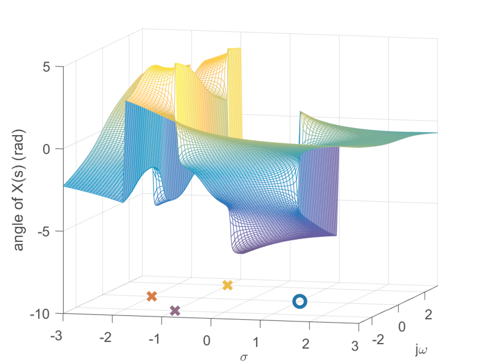
with ROC $\sigma >-1$, which corresponds to the intersection between the ROCs of individual parcels of $x(t)$. Figure 2.21 depicts the positions of the poles and zeros in the S-plane. And Figure 2.22 and Figure 2.23 show the magnitude (in dB) and phase of $X(s)$, respectively.

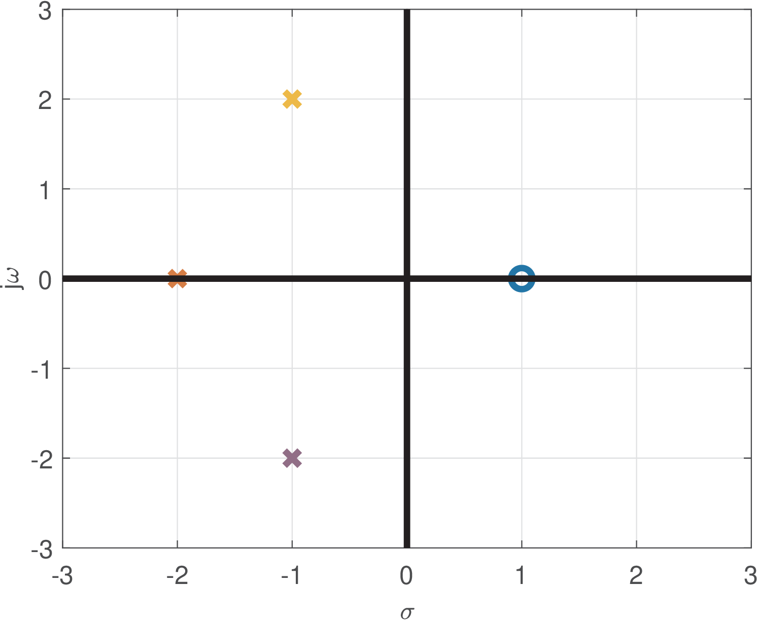
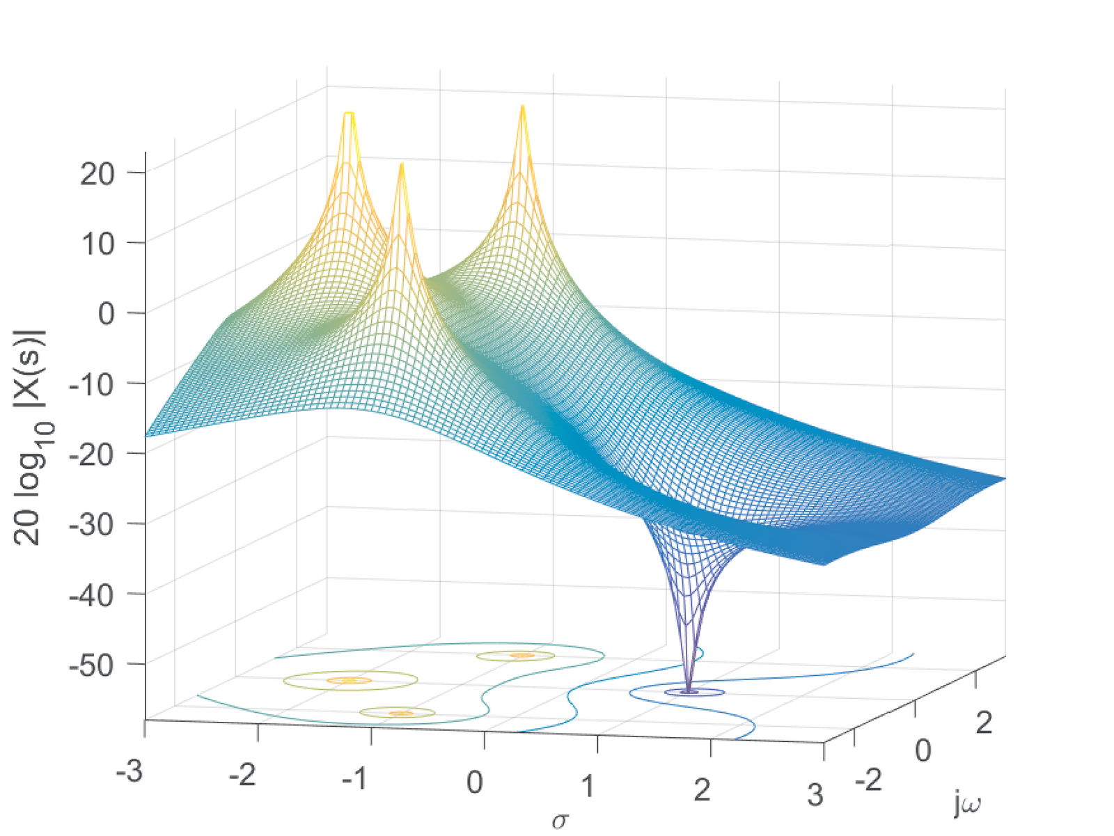
The values for which $X(s)=0$ are called zeros and the ones that lead to $X(s)=\infty$ are called poles. Figure 2.21 and Figure 2.22 provide complementary views of the positions of the zero at $s=1$ and the tree poles, as well as their impacts on the magnitude of $X(s)$. The locations of zeros appear as “valleys” while the poles are located at “volcanoes”. It is intuitive that the ROC cannot include poles because they are the positions for which $X(s)=\infty$, which violates “convergence”. For the example in Figure 2.22, the ROC is $\sigma >-1$ because $x(t)$ is right-sided and the right-most poles (assuming the orientation of the $\sigma$-axis is from $-\infty$ to $+\infty$) are at ${\sigma }_0=-1$.

Figure 2.23 shows the phase of $X(s)$. In most cases the phase is less instructive than the magnitude. Figure 2.23 emphasizes that the poles are conventionally signalized with “x” marks while zeros are represented by “o” marks.

The inverse Laplace transform can be obtained via partial faction decomposition (see Appendix A.10). Using the method residue in Python or Matlab/Octave is very convenient. For instance, in the case of Matlab/Octave:

1[r,p,k]=residue([1, -1], [1 4 9 10])

gives the residues r for each pole in p. This allows to write:

When all coefficients of $X(s)$ are real-valued, the pair of residues corresponding to complex conjugate poles are also complex conjugates. This is the case of the residues $0.3\pm j0.1$ in Eq. (2.55). By inspection of each of the three parcels and knowing $x(t)$ is causal, one can obtain the inverse transform as

It is convenient to expand the second (in blue) and third (in black) parcels and rewrite this equation as:

Grouping the parcels that can be written as a cosine and a sine, multiplying them by $2∕2$ and $2j∕(2j)$, and then using Eq. (A.1) (Euler’s formula), one can write $x(t)$ as:

This result can be obtained with symbolic math. For instance, using method ilaplace for the inverse Laplace transform in Matlab/Octave:

1syms s % define s as a symbolic variable 
2Xs = (s-1)/(s^3 + 4*s^2 + 9*s + 10) 
3xt = ilaplace(Xs) 
4pretty(simplify(xt))

These commands provide the same $x(t)$ calculated here.   $\text{□}$

An interesting fact is that the Laplace transform is a redundant representation and $x(t)$ could be eventually recovered from $X(s){|}_{\sigma ={\sigma }_1}$ if ${\sigma }_1$ is in the ROC. The following subsection will explore the possibility of finding the Fourier transform (if it exists) from the Laplace transform, by imposing the restriction of $\sigma =0$. From this Fourier transform, one can eventually recover $x(t)$, which illustrates the point that a Laplace transform has considerable redundancy in its representation of $x(t)$.

2.8.6  Calculating the Fourier transform from a Laplace transform

The Fourier transform basis function is equivalent to the Laplace’s when $\sigma =0$. Hence, the Laplace transform properties and pairs are similar to the Fourier ones.

Knowing that $X(s)=F\{x(t)e^{-\mathit{\sigma t}}\}$ the Fourier transform of $x(t)$ can be derived from its Laplace transform, i. e.,

in case $\sigma =0$ is in the ROC of $X(s)$ and, consequently, $x(t)$ has a Fourier transform.

Repeating this important result: Eq. (2.56) is valid only if the signal $x(t)$ has a valid Fourier transform. Using Example 2.21, note that the axis $\mathit{j\omega }$ is part of the ROC of $x(t)=e^{-2t}u(t)$, which then has a Fourier transform

In contrast, $x(t)=-e^{-2t}u(-t)$ does not have a valid Fourier transform: $X(\omega )$ does not converge and using Eq. (2.56) would lead to a wrong result!

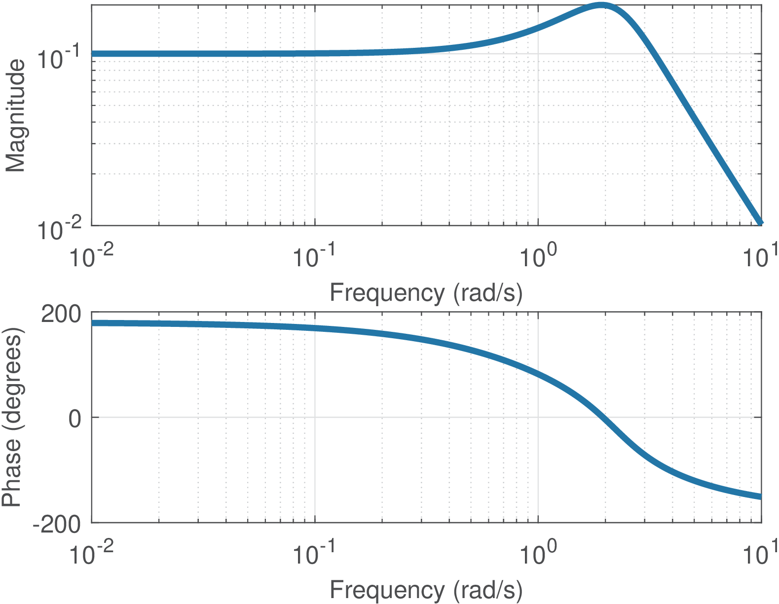
When the signal has both Fourier and Laplace transforms, a graph of $X(s)$ incorporates the corresponding graph of $X(\omega )$. Figure 2.24 shows the magnitude values for $s=\mathit{j\omega }$ (the $\mathit{j\omega }$ axis) as a curve in black, superimposed to Figure 2.22. Alternatively, Figure 2.25 shows only the values of $X(s)$ at the $s=\mathit{j\omega }$ axis.

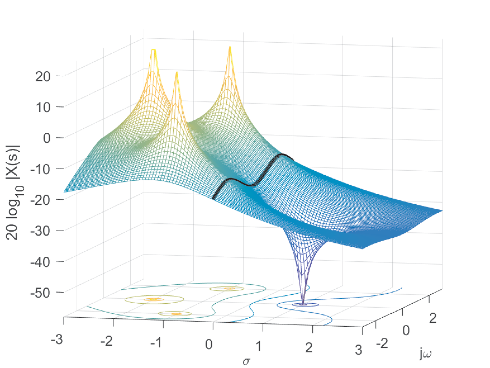
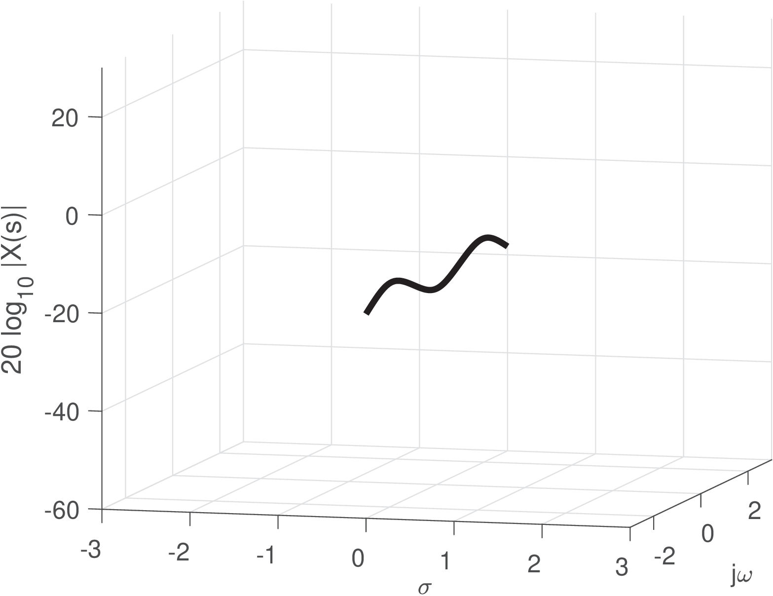
Both representations in Figure 2.24 and Figure 2.25 are three-dimensional and difficult to work with. Figure 2.26 depicts the frequency response in the conventional way, which is much easier to interpret than looking at Figure 2.25, for example. However, it is interesting to compare the figures and note that the peaks in Figure 2.26 are related to the position of the poles and draw conclusions such as that, the closer the pole is to the $\sigma =0$ axis, the more evident is the corresponding peak at the Fourier transform. In filter design, it is sometimes necessary to locate poles in the vicinity of the $\omega$ axis because this conducts to filters with high quality factor.

The need to use the Laplace as an alternative to the Fourier transform would be even greater if impulses were not allowed in Fourier analysis. The use of impulses in both the time and frequency domains allows a much larger class of signals to be represented with Fourier equations. For example, the ramp signal $x(t)=tu(t)$, strictly does not have a Fourier transform because the following integral does not converge:

However, using impulses, it is possible to use Fourier representations of signals such as $x(t)=tu(t)$, $x(t)=u(t)$ and $x(t)=\text{cos}<!--\; FUNCTION\; APPLICATION\; -->({\omega }_{0}t)$. This fact influences the main applications of the Laplace transform to be the representation of systems, not signals. For example, in terms of signals, while $x(t)=\text{cos}<!--\; FUNCTION\; APPLICATION\; -->({\omega }_{0}t)u(t)$ has the transform $X(s)=s∕(s^2+{\omega }_0^2)$, an infinite-duration sinusoid is not represented in the Laplace transform domain.

Because most signals that are analyzed with the Laplace transform are right-sided, sometimes the adopted definition is

which is called the unilateral Laplace transform (in contrast to the bilateral definition of Eq. (2.51)). Both coincide if the signal is right-sided (e. g., by the action of $u(t)$).