3.10 Introduction to Digital Filters
3.10.1 Designing simple filters using specialized software
Before studying digital filters in more details, it is useful to briefly discuss analog filters because most of the times they are required in digital signal processing systems as will be discussed here.
Example of analog filter design
There are integrated circuits (IC) that implement analog filters. They can also be built using discrete components: resistors, capacitors, inductors and operational amplifiers (opamps). The design of a filter corresponds to obtaining its system function. In the case of analog filters, there are many recipes (well-established algorithms, also called approximations) to obtain a system function that obeys the specified requirements in a project. The most common approximations are the Butterworth, Chebyshev, Bessel and Cauer (or elliptic).
Having , the next step is the realization of the filter using a circuit, i. e., establishing the topology and the components of the circuit that (approximately) implement . These two steps are the subject of many textbooks on filter design. Here, the approach will be to simply provide an example using the FilterPro software from Texas Instruments [ url3tif]. This software allows to obtain the schematic and components.14
Analog filters that use only resistor, capacitors and inductors are called passive filters. An alternative to avoid using inductors15 are active filters, which are typically based on opamps. When the target is an IC, not a circuit with discrete components, inductors are avoided due to the difficulty of their integration using current microelectronics technology. When an analog filtering operation is required in an IC, an active filter is typically adopted and this is the only class of filters supported by FilterPro.
Example 3.13. Example of analog filter designed with FilterPro. The following example illustrates the design of an analog filter with a desired cutoff frequency kHz, which is assumed to define the passband, such that the passband frequency is . A second-order lowpass filter with passband frequency of approximately 977.2 Hz was obtained with FilterPro and its schematic16 is shown in Figure 3.28.
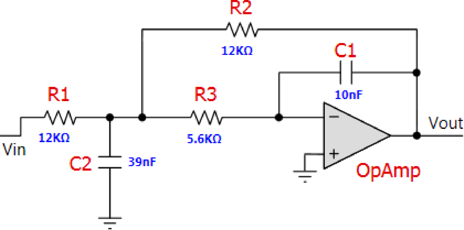
The system function can be obtained by analyzing the circuit in Figure 3.28. After that, can be compared to the ideal one obtained e. g. with Matlab/Octave via the command: [Bs,As]=butter(2,2*pi*1000,’s’) that gives
|
| (3.48) |
The arguments of the function butter are the filter order and the cutoff frequency in rad/s (not Hz). Note the required ’s’ to indicate to Matlab/Octave that the goal is to design an analog, not a digital filter.
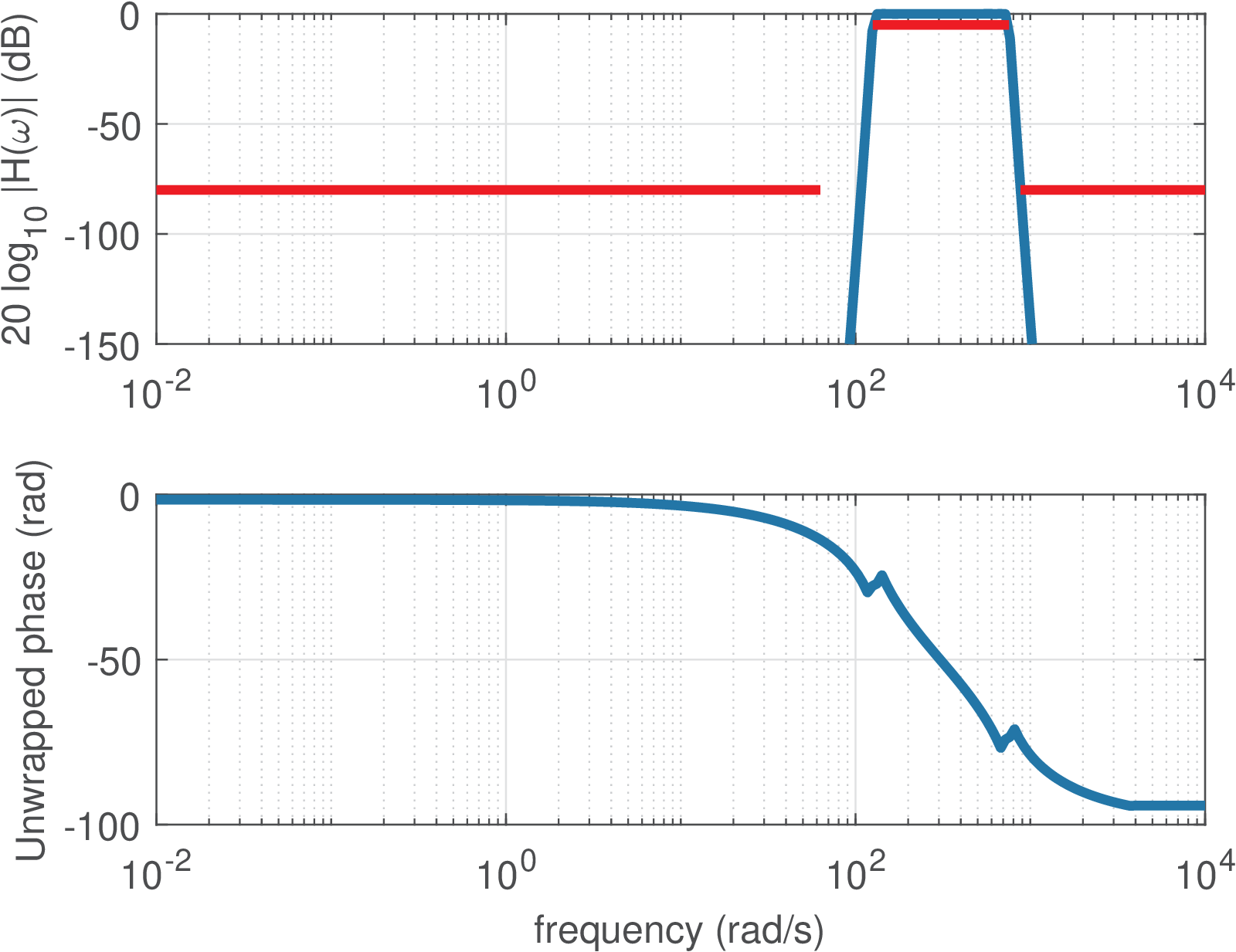
Example 3.14. Further examples of analog filter design in Matlab. Listing 3.11 illustrates how to design some analog filters with a given specification for its magnitude using Matlab (this code is not compatible with Octave). The frequency response magnitude and phase of the four designed filters are depicted in Figure 3.29.
1Apass=5; %maximum ripple at passband
2Astop=80; %minimum attenuation at stopband
3%% Lowpass Elliptic %%%%%%%%%
4Fp=100; Wp=2*pi*Fp; %passband frequency
5Fr=120; Wr=2*pi*Fr; %stopband frequency
6[N, Wp] = ellipord(Wp, Wr, Apass, Astop, 's') %find order
7[z,p,k]=ellip(N,Apass,Astop,Wp,'s'); %design filter
8B=k*poly(z); A=poly(p); %convert zero-poles to transfer function
9[H,w]=freqs(B,A); %calculate frequency response
10%% Higpass Elliptic %%%%%%%%%
11Fr=100; Wr=2*pi*Fr; %stopband frequency
12Fp=120; Wp=2*pi*Fp; %passband frequency
13[N, Wp] = ellipord(Wp, Wr, Apass, Astop, 's') %find order
14[z,p,k]=ellip(N,Apass,Astop,Wp,'high','s'); %design filter
15B=k*poly(z); A=poly(p); %convert zero-pole to transfer function
16[H,w]=freqs(B,A); %calculate frequency response
17%% Bandpass Elliptic %%%%%%%%
18Fr1=10; Wr1=2*pi*Fr1; %first stopband frequency
19Fp1=20; Wp1=2*pi*Fp1; %first passband frequency
20Fp2=120; Wp2=2*pi*Fp2; %second passband frequency
21Fr2=140; Wr2=2*pi*Fr2; %second stopband frequency
22[N,Wp]=ellipord([Wp1 Wp2],[Wr1 Wr2],Apass,Astop,'s') %find order
23[z,p,k]=ellip(N,Apass,Astop,Wp,'s');%design filter
24B=k*poly(z); A=poly(p); %convert zero-pole to transfer function
25[H,w]=freqs(B,A); %calculate frequency response
26%% Bandpass Butterworth %%%%%%%%%%%
27[N, Wn]=buttord([Wp1 Wp2],[Wr1 Wr2],Apass,Astop,'s')%find order
28[z,p,k]=butter(N,Wn,'s'); %design Butterworth filter
29B=k*poly(z); A=poly(p); %convert zero-pole to transfer function
30[H,w]=freqs(B,A); %calculate frequency response
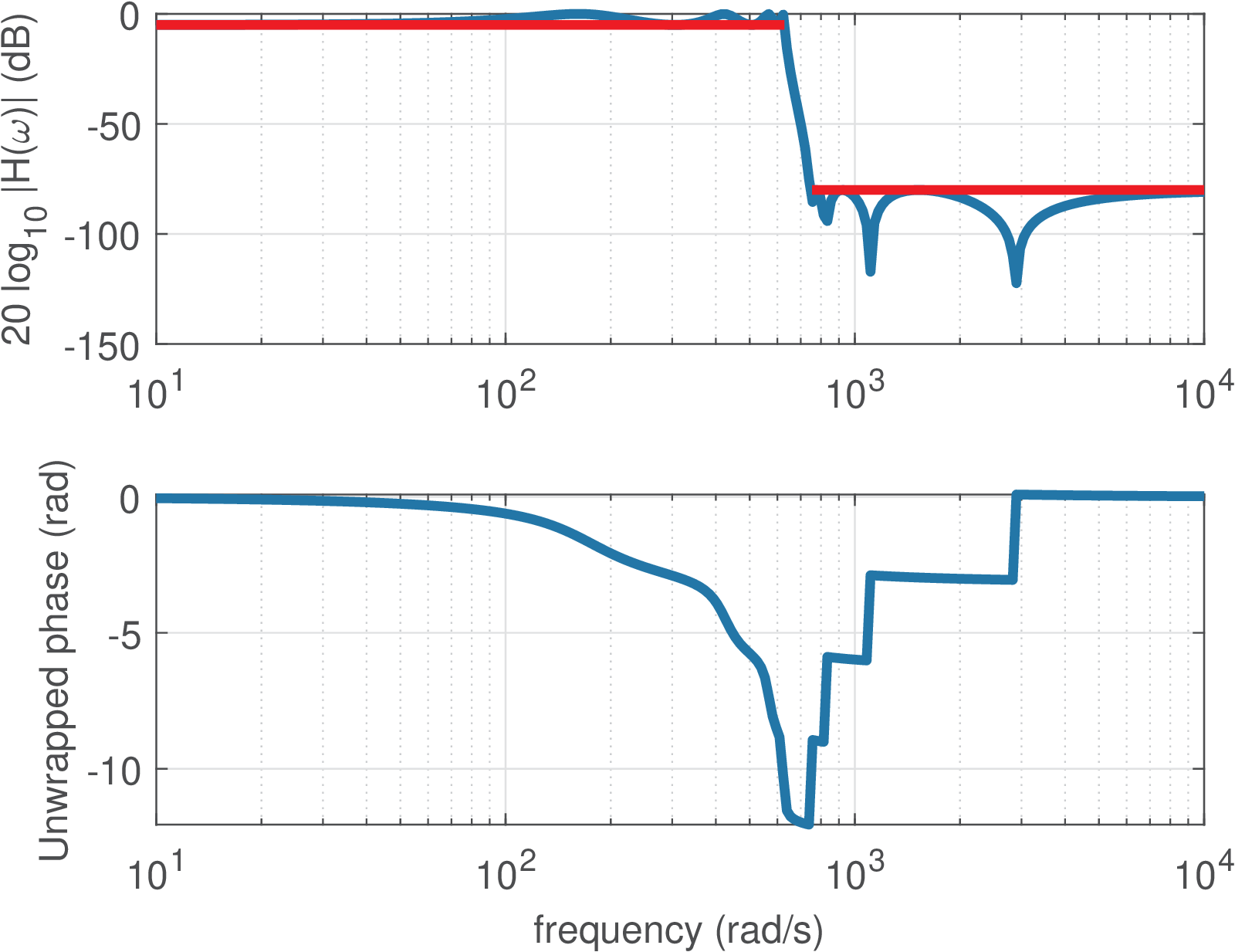
(a)
Lowpass
elliptic
(). |
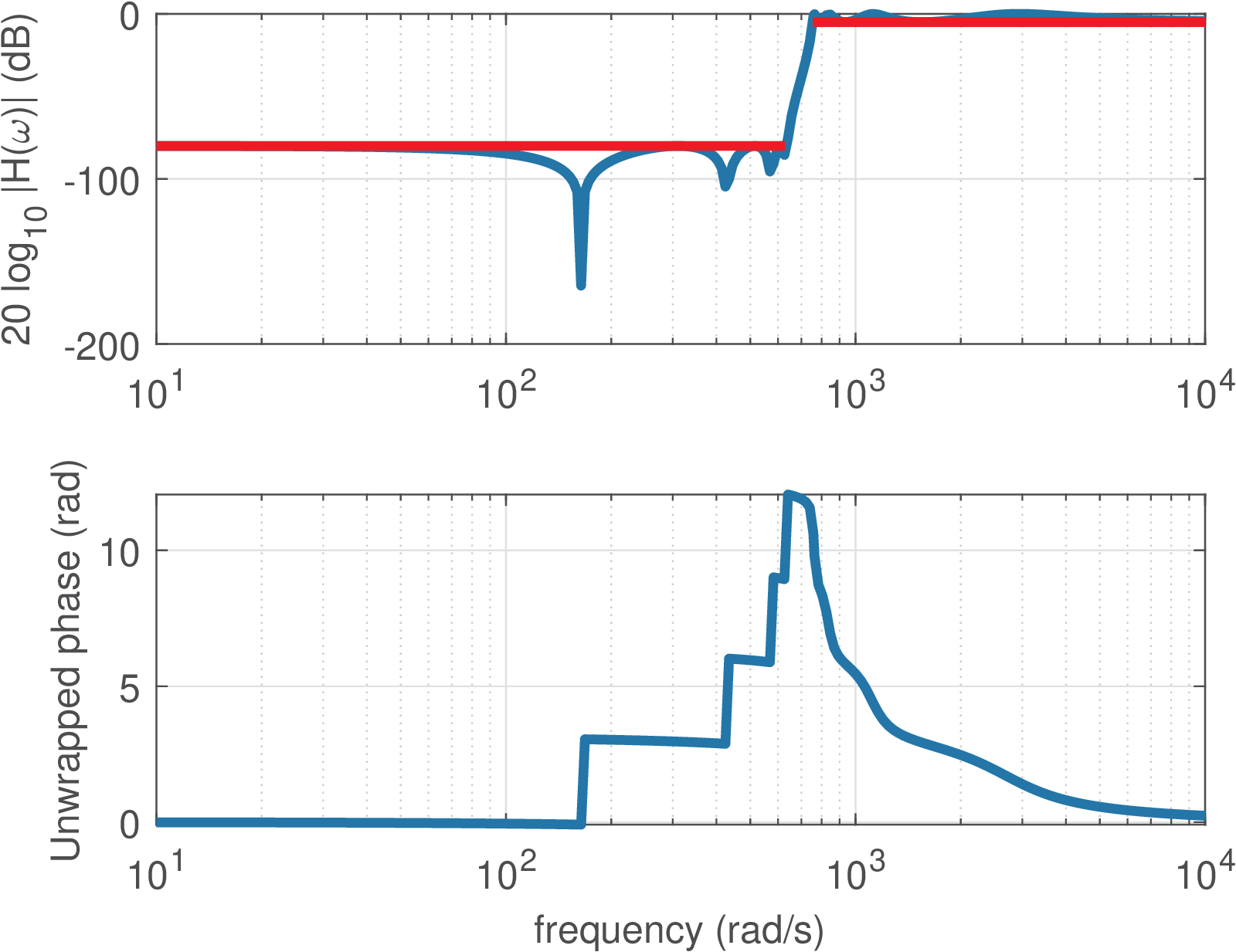
(b)
Highpass
elliptic
(). |
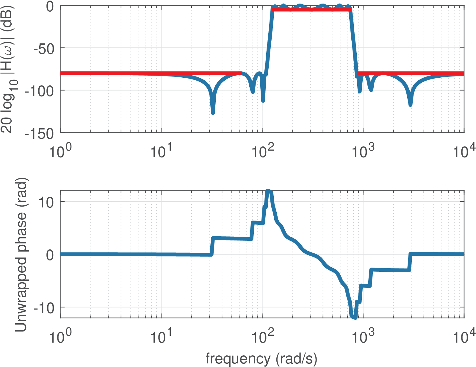
(c)
Bandpass
elliptic
(). |
(d)
Bandpass
Butterworth
(). |
It should be noted from Listing 3.11 and Figure 3.29 that a bandpass filter has twice the order that is specified as an input parameter (and obtained by buttord and ellipord in this example). Note also that, in practice, an analog filter typically has an order between 1 to 10. For example, an order is not feasible for practical implementation with an analog circuit.
Example of digital filter design

For comparison, it is interesting to design now an equivalent digital filter to substitute its analog counterpart corresponding to . But in order to interface with the external (analog) world, four extra blocks are required, as illustrated in Figure 3.30. The filters (anti-aliasing) and (external reconstruction) are lowpass analog filters with passband frequency equal to half of the sampling frequency, which is assumed here to be kHz. Their gains are not important at this moment and in practice they are determined by the interfacing electronics. Assuming the converters and analog filters are properly defined, it remains to design , which can be done with the command
that leads to
|
| (3.49) |
It is important to note that when designing an analog filter, the second argument of butter is in rad/s. For a digital filter, as explained in Section 1.8.4, Matlab/Octave uses the normalized frequency . In this case, the Nyquist frequency is 5 kHz and using Eq. (1.41), Hz is normalized by the Nyquist frequency in the command [Bz,Az]=butter(2,(1000/5000)).
It will be later discussed in this chapter that the function butter used the bilinear transformation to convert of Eq. (3.48) into of Eq. (3.49).
From Table 3.1 one knows the definition and this should not be confused with in Eq. (3.49). In many applications is a rational function (a ratio of two polynomials), with specifying the numerator and the denominator. In general, and .
Digital filters described by a rational function can be conveniently implemented via a LCCDE, as discussed next.
Example 3.15. Obtaining the difference equation and implementing a digital filter. For example, assume that a LTI system with impulse response outputs when the input is . In this case, and , which leads to with and . With this concept in mind, Eq. (3.49) can be written as
and taking the Z-inverse one can obtain the difference equation corresponding to Eq. (3.49):
The amazing fact is that this can be implemented with a simple code, similar to Listing 3.12.
1initialization() { %all previous values are assumed 0
2    xnm1=0 %variable to store the value of x[n-1]
3    xnm2=0 %x[n-2]
4    ynm1=0 %y[n-1]
5    ynm2=0 %y[n-2]
6}
7processSample() {
8    xn=readFromADConverter() %read input sample from ADC
9    yn=0.067455*xn + 0.134911*xnm1 + 0.067455*xnm2 +
10       1.14298 ynm1 - 0.41280 *ynm2
11    writeToDAConverter(yn) %write output sample into DAC
12    ynm2=ynm1 %update for next iteration. Note the order of ...
13    ynm1=yn   %updates: avoid overwriting a value ...
14    xnm2=xnm1 %that should be used later
15    xnm1=xn
16}
where one assumes a timer17 invokes the function processSample at a rate of (10 kHz in this case).
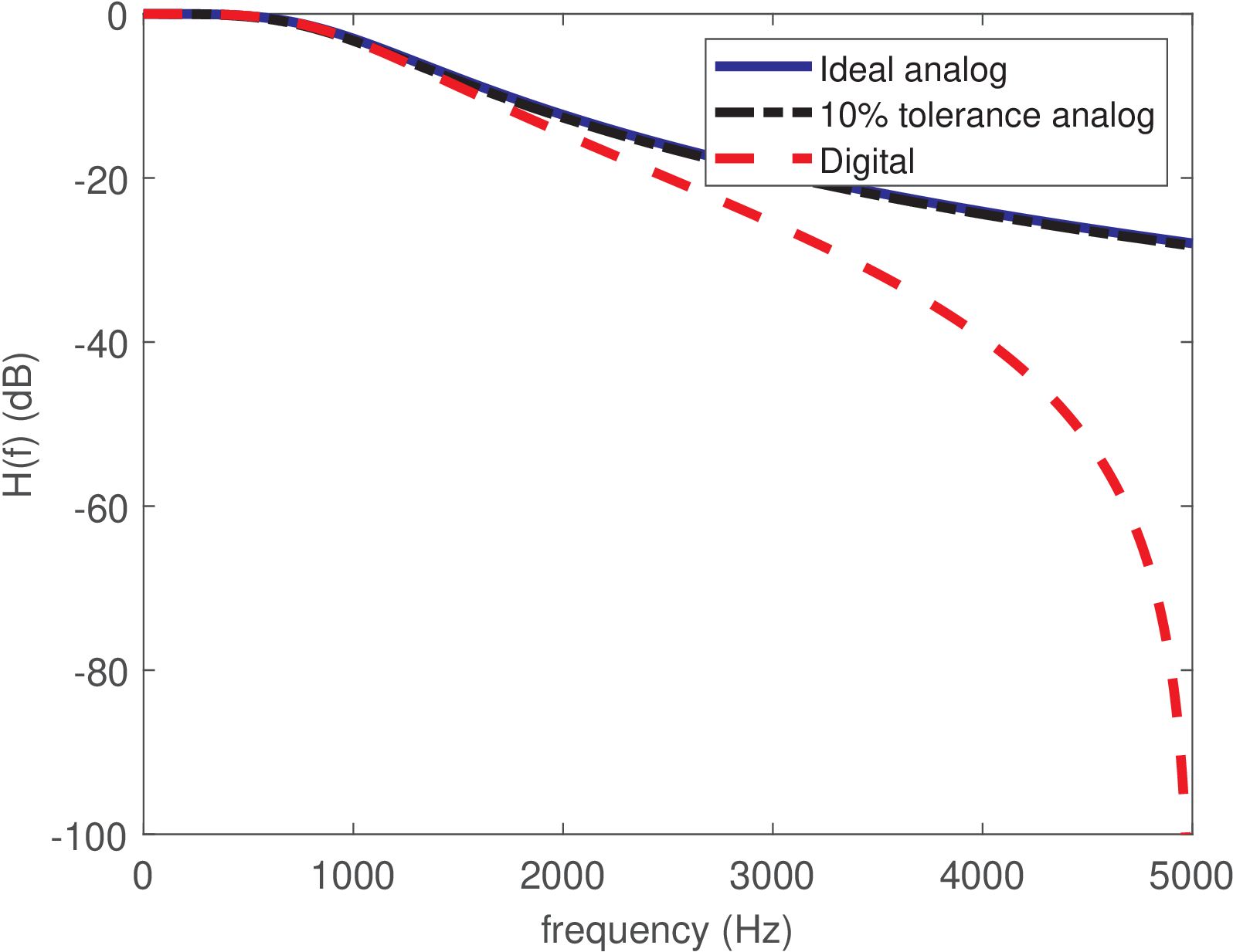
Figure 3.31 compares the discussed filters, illustrating that has a lowpass frequency response that is similar in terms of passband frequency to the original . For frequencies above the passband, attenuates more than , but this is not deleterious for a lowpass filter. Later, in Section 3.12.4, this behavior will be clarified, which is intrinsic of having the bilinear transformation mapping the behavior of the analog filter at infinite frequencies into rad (or Hz) for , i. e., mapping into .
If is changed, the frequency response of the overall system in Figure 3.30 is scaled according to (Eq. (1.37)). For example, decreasing from 10 to 5 kHz would divide by two the cutoff frequency of the overall system.
3.10.2 Distinct ways of specifying the “ripple” deviation in filter design
As illustrated in Figure 3.29, practical filters have a frequency response that deviates from the ideal ones. Instead of a flat magnitude over the whole passband and zero gain in the stopband, as depicted in Figure 3.1, a non-ideal filter has deviations from the target values and eventual “oscillations” called “ripples”. When designing a filter, it is possible to impose limits to these ripples, but this procedure is different for the passband and stopband “ripples” / deviations, as discussed next.
There are several ways of specifying the maximum “ripple” or deviation at the passband of a filter. For example, it can be specified in dB or linear scale, which are called here and , respectively (as suggested by Matlab). If one assumes a lowpass filter with a unitary gain at DC, the maximum linear deviation can be assumed to be within or . The latter option is particularly useful if the filter magnitude monotonically decreases as for the Butterworth filters and is assumed here, meaning that the frequency response is 1 at DC and decreases in the passband to a value not smaller than . For example, a specification can be that the passband magnitude does not deviate 5% of the gain at DC. In this case, and the minimum magnitude at passband is . Often, this value is specified in dB as
If the deviation is within in linear scale, then it is confined to in dB.
At the stopband, the magnitude in linear scale is also a “deviation” because the reference value is 0 (the desired magnitude at stopband). In other words, for the stopband, the deviation coincides with the magnitude itself and its value in dB is given by
Often, the filter magnitude has a maximum value of 0 dB and the values of and are positive.
Matlab uses the same convention adopted here in its routines. This is exemplified in Listing 3.13, which uses the method buttord to find the order of a Butterworth filter that complies with the project specifications.
1Wp=0.3; %normalized passband frequency (rad / pi)
2Ws=0.7; %normalized stopband frequency (rad / pi)
3Rp=1; %maximum passband ripple in dB
4Rs=40; %minimum stopband attenuation in dB
5[n,Wn] = buttord(Wp,Ws,Rp,Rs); %find the Butterworth order
6[B,A]=butter(n,Wn); %design the Butterworth filter
7zp=exp(1j*pi*Wp); zs=exp(1j*pi*Ws); %Z values at Wp and Ws
8%% Check if the filter obeys requirements
9linearMagWp = abs(polyval(B,zp)/polyval(A,zp)) %mag. at Wp
10linearMagWs = abs(polyval(B,zs)/polyval(A,zs)) %mag. at Ws
11Dp_result = 1-linearMagWp %linear deviation at Wp (linear)
12Rp_result = -20*log10(1-Dp_result) %deviation (ripple) at Wp (dB)
13Ds_result = linearMagWs %linear deviation at Ws (linear)
14Rs_result = -20*log10(Ds_result) %deviation (ripple) at Ws (dB)
The required filter order is n=4, and the obtained results are: linearMagWp=0.9105, linearMagWs=0.01, Dp_result=0.0895, Rp_result=0.8147, Ds_result=0.01 and Rs_result=40.0. They can be interpreted as follows. Matlab designed the method buttord to meet exactly the requirements for the stopband, while giving an eventual slack to the requirements for the passband. Hence, we can see that Rs_result=40.0 dB is exactly the specified attenuation at the stopband. This corresponds to a linear gain linearMagWs=0.01 of the filter’s frequency response at the beginning of the stopband. Using mathematical notation: in linear scale, which corresponds to dB.
The filter gain is 1 at DC, and it decreases until reaching linearMagWp=0.9105 in the end of its passband. In our notation, , which corresponds to dB. This value does not coincide with Rp_result=0.8147 due to the rounding to four decimal places. Using 20*log10(linearMagWp) gives the precise gain value of dB. Note that the deviation in the passband of 0.8147 dB from the ideal 0 dB is within the maximum value of 1 dB imposed to buttord. There is a slack of dB.
In summary, it is a bit confusing how Matlab and other software define the input parameters to functions such as buttord. But one just needs to interpret the ripples in dB as obtained from “deviations” of the ideal values of 1 and 0 in passband and stopband, respectively.
3.10.3 LCCDE digital filters
A digital filter is a discrete-time system that deals with quantized input and output signals (quantized amplitudes). A possible practical scenario for a digital filter is the one shown in Figure 3.30. There are many different kinds of digital filters but this section assumes filters that are based on linear constant-coefficient difference equations (LCCDE). As indicated in Figure 3.5, when zero initial conditions are assumed, the LCCDE systems are a special case of LTI systems. But when one takes in account the non-linear quantization effects that occur in practical CPUs (or digital signal processors) due to their limited precision, the overall system is not strictly LTI. In spite of that, it is convenient to isolate the effects of quantization and finite-precision arithmetics, and study digital filters as LTI LCCDE systems. Later on, the impact of quantizing the filter coefficients and the roundoff errors due to finite-precision can be incorporated. Therefore, hereafter, the term digital filter refers to discrete-time LTI LCCDE systems. Besides, the systems are assumed to be causal.
A system that has the output and input signals related by a LCCDE such as
|
| (3.50) |
can be represented by (taking the Z-transform on both sides of the LCCDE)
In this case, the transfer function is
|
| (3.51) |
which, after eventual algebraic simplifications, can be written as the ratio
|
| (3.52) |
of two polynomials in . Calculating the zeros (roots of the numerator ) and the poles (roots of the denominator ), one can write
where is a gain. The coefficients of Eq. (3.50) can be real or complex. For simplicity, they will be assumed real () unless otherwise stated. In this case, and the roots are real or, for each root , its complex conjugate is also a root such that the product leads to a second-order polynomial with real coefficients.
It is useful to know that the value of at and correspond to the values of the frequency response at (DC) and rad, respectively, which can be written as
|
| (3.53) |
For example has a frequency response with and .
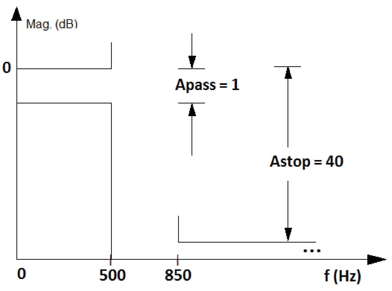
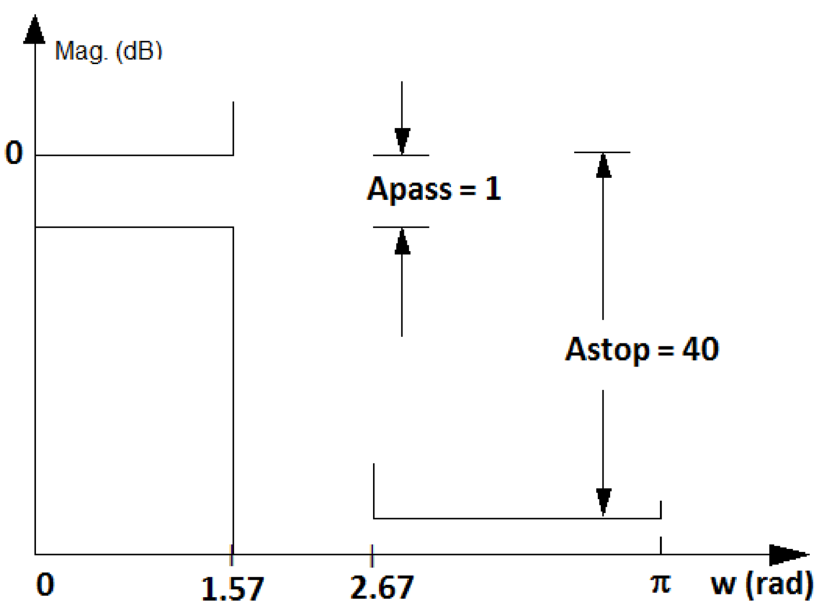
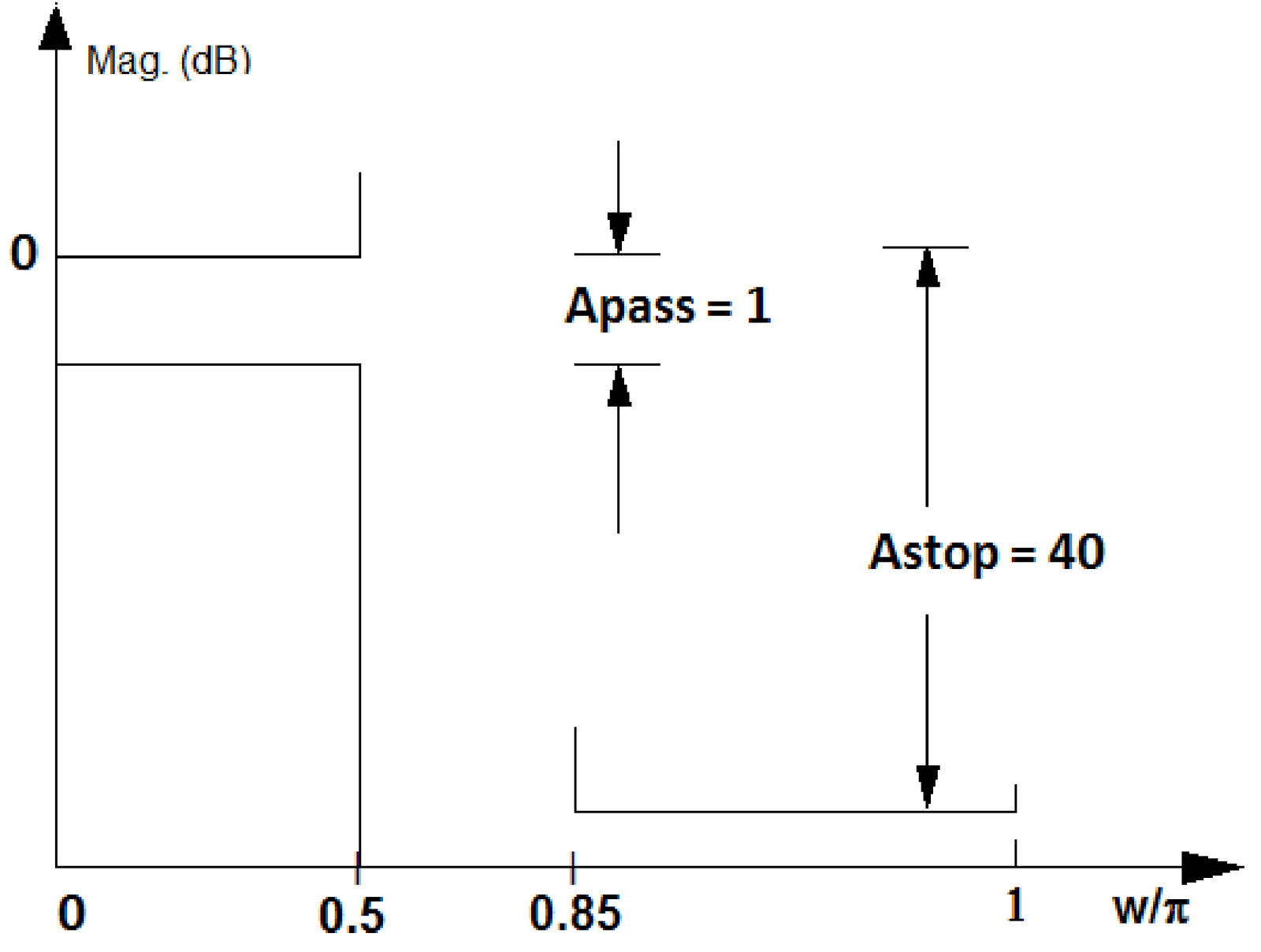
Example 3.16. Specifying a filter in Hz, rad or normalized frequency. When designing digital filters, it is important to remember the fundamental relation , first presented in Eq. (1.37). Figure 3.32 illustrates how this relation can be used to convert a specification for a lowpass analog filter with passband and stopband frequencies of 500 and 850 Hz, respectively, into a specification of a digital filter with , which leads to passband and stopband frequencies of and rad, respectively.
(a)
Analog
(
in
Hz) |
(b)
Digital
(
in
rad) |
(c)
Digital
(
in
) |
Figure 3.32 also shows the convention used by Matlab/Octave, which gets rid of the irrational number by using a normalized axis , as listed in Table 1.5. In this case, can be written as , which simplifies to obtaining with the normalization of by the Nyquist frequency . For example, Hz in Figure 3.32(a) turns into in Figure 3.32(c). This normalization by the Nyquist frequency is sensible because digital filters are always constrained to work with frequencies of at most Hz, which corresponds to rad.
3.10.4 FIR, IIR, AR, MA and ARMA systems
An important characteristic of a digital filter is the duration of its impulse response, which allows to classify it as a finite impulse response (FIR) or infinite impulse response (IIR) filter. For example, a filter with is FIR and a filter with is IIR. Note that if one plots in a computer, due to the limited precision, the values of would underflow to zero for large enough , but theoretically this impulse response has infinite duration.
Another characteristic is whether the filter is recursive or not. A recursive filter has the output depending on past values of the output itself () while the output of a non-recursive filter depends only on the input and its past values (assuming causality). The system function of a non-recursive filter has in Eq. (3.51) and no finite poles.
In practice, FIR can be associated to non-recursive filters and IIR to recursive filters. But recursiveness and impulse response duration are two distinct concepts! It is possible to create a recursive filter with an impulse response of finite duration using cancellation of poles and zeros, for example. In spite of that, the design of recursive filters is often called “IIR design”. Similarly, “FIR design” is the topic that concerns the design of non-recursive filters. This widely adopted jargon is used in this text.
IIR and FIR filters will be discussed in the sequel. While the subject is presented in the context of digital filtering, many conclusions are valid for systems in general. In other words, IIR and FIR systems can be found in applications in which the goal is not filtering, but system identification, equalization, control, tracking, statistics, etc. In some of these areas, is not classified as FIR or IIR, but as MA, AR or ARMA “model”.
A moving-average (MA) model is a non-recursive FIR filter and an autoregressive (AR) filter is a special case of a recursive IIR filter for which in Eq. (3.51). The AR IIR filter does not have finite zeros other than at the origin and is given by
|
| (3.54) |
Note in Eq. (3.54) that the gain value for the numerator is chosen such that the denominator coefficient of Eq. (3.51) is equal to 1. The numerator leads to zeros at and makes causal.
The autoregressive-moving-average (ARMA) model is a generic model composed by an AR (denominator) and MA (numerator) sections. There are many generalizations of these basic models, which are adopted in areas such as statistics. Parametric modeling is the task of, according to a predefined criterion such as least-squares, fit the data to the assumed model. In spite of being defined in distinct scenarios, filter design and parametric modeling share several fundamental results.
Before discussing the design of IIR and FIR filters, it is useful to note the importance of frequency scaling.
3.10.5 Filter frequency scaling
Computational routines often produce a prototype with normalized frequencies (e. g., a cuttof frequency of 1 rad/s) that are then converted (eventually by another routine) to the required frequencies via frequency scaling.
With frequency scaling one can modify a filter to obtain a different cutoff frequency. For example, if has a cutoff of rad/s, the transformation moves this cutoff frequency to rad/s. The operation is similar to using to double the “speed” of a signal represented by , which leads to having half of the support of . Similarly, has twice the support of . More specifically, if the prototype has a cutoff frequency of 1 rad/s, then
|
| (3.55) |
scales the complex plane, and consequently , such that is the cutoff frequency of the new filter .
There are computational routines that provide a prototype filter with (normalized) cutoff frequency of rad/s, which can then be converted to a new filter with an arbitrary cutoff frequency with the transformation . For example, this change in cutoff frequency can be done in Matlab by applying the function lp2lp to a lowpass analog prototype (current version of Octave misses this functionality) as indicated in Listing 3.14.
1N = 5; %filter order
2[B,A] = butter(N,1,'s'); %prototype with cutoff=1 rad/s
3[Bnew,Anew]=lp2lp(B,A,100); %convert to cutoff=100 rad/s
4freqs(Bnew,Anew) %plot mag (linear scale) and phase
Note that lp2lp requires the prototype to have a cutoff frequency of rad/s (besides being an analog lowpass filter).
Example 3.17. Frequency conversion when the prototype does not have a cutoff frequency of 1 rad/s. Assume that a frequency conversion must be applied to such that its cutoff frequency of rad/s is shifted to 30 rad/s. Because this is a simple first-order filter, the final result can be immediately obtained. But the whole procedure is described because it is useful for higher-order filters.
A convenient step is to move the cutoff frequency of to 1 rad/s using a substitution of by , which leads to
Now, the final filter can be obtained by expanding to 30 by substituting in by :
Alternatively, one could directly use . These frequency conversions are widely used in the design of IIR filters as will be discussed.
3.10.6 Filter bandform transformation: Lowpass to highpass, etc.
There are many transformations to convert a prototype (or reference) filter into another one. Section 3.10.5 briefly discussed frequency scaling. It is also possible to convert a lowpass prototype filter into a highpass, bandpass and bandstop, for example, which is called bandform transformation.
When dealing with analog filters, it is often necessary to apply impedance scaling to have the filter input and/or output with a desired impedance. The intent in this case is not to change the transfer function, but to perform impedance matching. All these three kinds of filter transformations are well-discussed in the literature18. In the sequel, bandform transformation is briefly discussed.
Bandform transformations can be used to create a bandpass from a lowpass prototype, for example. These transformations differ considerably for analog and digital frequencies, especially due to the fact that a digital filter has a periodic spectrum.19 Having a lowpass analog prototype, a Matlab user20 can use the functions lp2bp, lp2bs and lp2hp to convert it to bandpass, bandstop and highpass filters, respectively.
Sometimes frequency scaling is incorporated to bandform transformation such that a routine converts a lowpass prototype with normalized 1 rad/s cutoff frequency into another filter with desired bandwidth and frequencies. For example, the Matlab’s function lp2bp converts a normalized lowpass into a bandpass with the desired center frequency and bandwidth as illustrated in Listing 3.15.
1N = 4; %prototype order (bandpass order is 2N = 8)
2[B,A] = butter(N,1,'s'); %prototype with cutoff=1 rad/s
3[Bnew,Anew]=lp2bp(B,A,50,30); %convert to cutoff=50 rad/s
4freqs(Bnew,Anew) %plot mag (linear scale) and phase
The functions lp2bp, lp2bs, lp2hp and lp2lp are restricted to analog filters. Transformations of digital filters can be achieved via a mapping provided by allpass filters, which are filters that have unitary magnitude for all frequencies and just change the phase of the input signal. Besides frequency transformation, allpass filters are adopted for phase equalization and other applications. Some Matlab functions that provide support to digital filter transformations are iirlp2bs, iirlp2bp, iirlp2xn, iirftransf, allpasslp2xn and zpklp2xn.
For example, Listing 3.16 compares the conversion of a Butterworth and a elliptic lowpass prototypes, both with cutoff frequency rad, into stopband versions with cutoff frequencies and rad. The two prototypes are halfband filters because their cutoff frequencies is rad.
1Wc=0.5; %cutoff (normalized) frequency of prototype filter
2Wstop = [0.5 0.8]; %stopband cutoff frequencies
3N=3; %order of prototype filter
4[B,A] = butter(N,Wc); %Butterworth prototype
5[Bnew,Anew]=iirlp2bs(B,A,Wc,Wstop); %Bandstop Butterworth
6[B2, A2] = ellip(N, 3, 30, Wc); %Elliptic prototype
7[Bnew2,Anew2]=iirlp2bs(B2,A2,Wc,Wstop); %Bandstop elliptic
8fvtool(Bnew2, Anew2, Bnew, Anew); %compare freq. responses
For the comparison, it was used the Matlab’s Filter Visualization Tool (fvtool). Note that the fourth argument of ellip is the passband frequency (not necessarily the cutoff frequency). In this case, a maximum ripple of 3 dB was specified using the second argument of ellip to have the passband frequency coinciding with the cutoff frequency Wc ( rad). Besides, a minimum attenuation of dB was required for the stopband of the elliptic lowpass prototype.
As another example, the following Matlab code converts a Butterworth lowpass prototype with cutoff frequency rad into a bandpass with cutoff frequencies and rad.
1N = 5; %filter order
2[B,A] = butter(N,0.5); %prototype with cutoff=0.5 rad
3[Bnew,Anew]=iirlp2xn(B,A,[-0.5 0.5],[0.25 0.75],'pass');
The third and fourth arguments of function iirlp2xn ([-0.5 0.5] and [0.25 0.75]) indicate frequency points in the original filter and to what frequencies they should be mapped. In this case, rad should be mapped to rad and to rad.
Instead of creating a prototype and then converting to the desired filter, most routines allow to directly design the filter. The following commands illustrate the design of highpass, bandpass and bandstop elliptic filters.
1N=5; %filter order for the lowpass prototype (e.g., bandpass is 2*N)
2Rp=0.1; %maximum ripple in passband (dB)
3Rs=30; %minimum attenuation in stopband (dB)
4[B,A]=ellip(N,Rp,Rs,0.4,'high'); %highpass, cutoff=0.4 rad
5[B,A]=ellip(N,Rp,Rs,[0.5 0.8]); %bandpass, BW=[0.5, 0.8], order=2*N
6[B,A]=ellip(N,Rp,Rs,[0.5 0.8],'stop'); %BW=[0.5, 0.8], order=2*N
Similarly, FIR design routines provide support to directly designing filters other than lowpass ones. For example, Listing 3.18 designs a stopband filter. Note the normalization by the Nyquist frequency Fs/2.
1Fs = 44100; %sampling freq. (all freqs. in Hz)
2N  = 100;   %filter order (N+1 coefficientes)
3Fc1  = 8400;  % First cuttof frequency
4Fc2  = 13200; % Second cuttof frequency
5B  = fir1(N, [Fc1 Fc2]/(Fs/2), 'stop', hamming(N+1));
Because there are plenty of routines for bandform transformation, the discussion about IIR and FIR filter design concentrates on lowpass filters.