Realization of Digital Filters

3.15 Realization of Digital Filters

Having $H (z)$ , the next step is to choose a realization. For example, the difference equation $y [n] = 5 x [n] - 5 x [n - 1]$ could be implemented as $y [n] = 5 (x [n] - x [n - 1])$ to save computation. In this case, instead of two multiplications followed by a subtraction, the alternative requires only one subtraction and one multiplication. However, a difference equation is not adequate to distinguish realizations. For example, algebraically, they are of course the same: $y [n] = 5 x [n] - 5 x [n - 1] = 5 (x [n] - x [n - 1])$ . In order to specify realizations of digital filters, a flow chart or diagram is used. The “delay block” is represented by $z^{- 1}$ , such that its output is the previous value of the input. For example:

x [n] \to z^{- 1} \to x [n - 1]

and

y [n] \to z^{- 1} \to z^{- 1} \to z^{- 1} \to y [n - 3] .

The output of each delay block needs to be stored in RAM memory, such that the number of delay blocks should be minimized if one aims at minimizing memory consumption. The filter memory is the set of values taken from the output of the delay blocks, which are stored for using in the next iteration.

Other blocks are the multiplier and adder. These three help to indicate the order of operations when implementing a difference equation. Figure 3.53 depicts the two realizations mentioned previously. A careful observation concludes that such diagrams still have some ambiguity with respect to the order of operations but they are more descriptive than a difference equation.

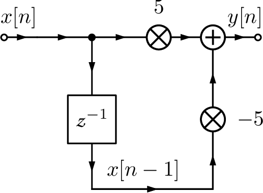
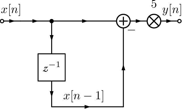
Figure 3.53: Two distinct realizations of $y [n] = 5 x [n] - 5 x [n - 1]$ .

At this point, it may not be clear that the value of $y [n]$ can be distinct in the two cases of Figure 3.53. This may happen when one compares these two filter realizations using a finite number of bits to represent numbers. For example, assume that the hardware used to implement the equations provides only 8 bits to represent integer numbers in the range $[- 128, 127]$ in two’s complement. Say that $x [0] = 85$ and $x [1] = 92$ and the goal is to obtain $y [1]$ . Using the realization of Figure 3.53(b), the difference $x [1] - x [0] = 92 - 85 = 7$ is multiplied by 5 and $y [n] = 35$ . In contrast, using Figure 3.53(a) leads to an overflow when calculating $5 x [0] = 425$ , which would require at least 10 bits because converting from decimal to binary leads to $42 5_{D} = 01 1010 100 1_{B}$ , with the most significant bit representing the sign. Therefore, unless the hardware was able to implement saturation and represent this product as 127, the result with finite precision would be $5 x [0] = - 8 7_{D} = 1010 100 1_{B}$ . Similarly, $5 x [1] = - 52$ when represented with 8 bits and, consequently, $y [1] = - 87 - (- 52) = - 35$ in this case. This simple example should suffice to illustrate the importance of the filter realization when the precision is finite. There are many structures for obtaining realizations of digital filters. The most popular will be presented in the sequel.

3.15.1 Structures for FIR filters

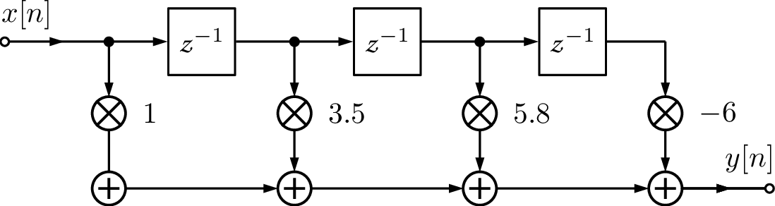
Figure 3.54: Two structures for FIR realizations.

The most straightforward implementation of a FIR is called direct form or tapped delay line, which is depicted in Figure 3.54(a) for $H (z) = 1 + 3.5 z^{- 1} + 5.8 z^{- 2} - 6 z^{- 3}$ .

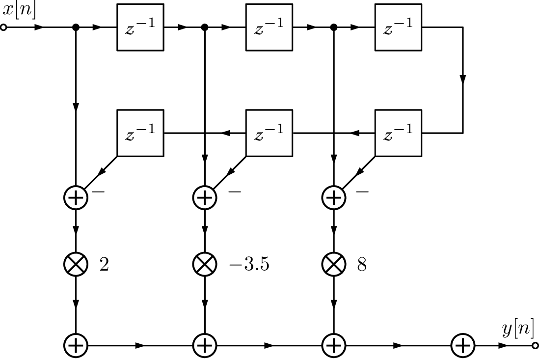
Many FIR filters are designed to have linear phase and, consequently, have symmetry in their coefficients,³⁶ as indicated in Table 3.9. This has been taken into account in the symmetric FIR structure of Figure 3.54(b), which implements $H (z) = 2 - 3.5 z^{- 1} + 8 z^{- 2} - 8 z^{- 4} + 3.5 z^{- 5} - 2 z^{- 6}$ .

3.15.2 Structures for IIR filters

Figure 3.55: Two alternatives for implementing the digital filter of Eq. (3.97).

IIR filters are often implemented using the transposed direct II structure. It is convenient first to describe the direct I structure via an example. Assume the task is to implement:

H (z) = \frac{B (z)}{A (z)} = \frac{0.6 + 0.1 z^{- 1} + 2.3 z^{- 2} + 4.5 z^{- 3}}{1.0 - 1.2 z^{- 1} + 0.4 z^{- 2} + 5.2 z^{- 3} + 1.1 z^{- 4}} .

(3.97)

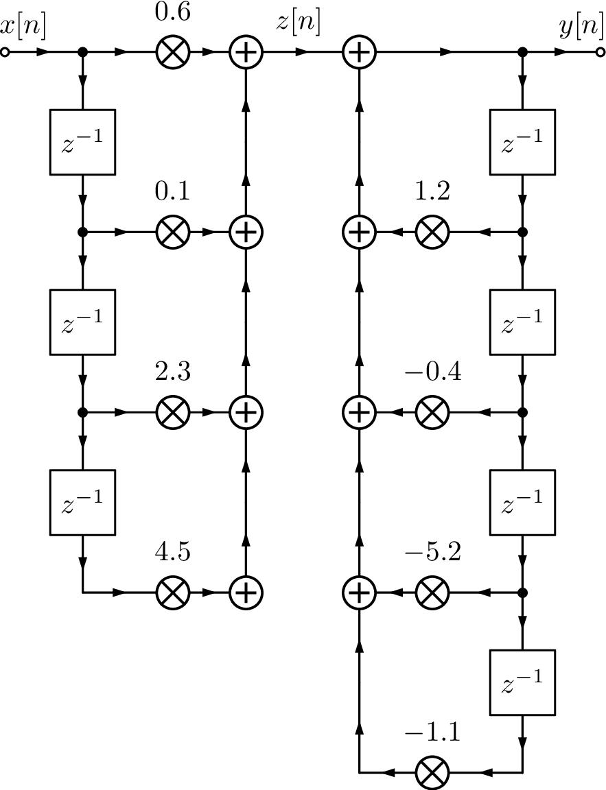
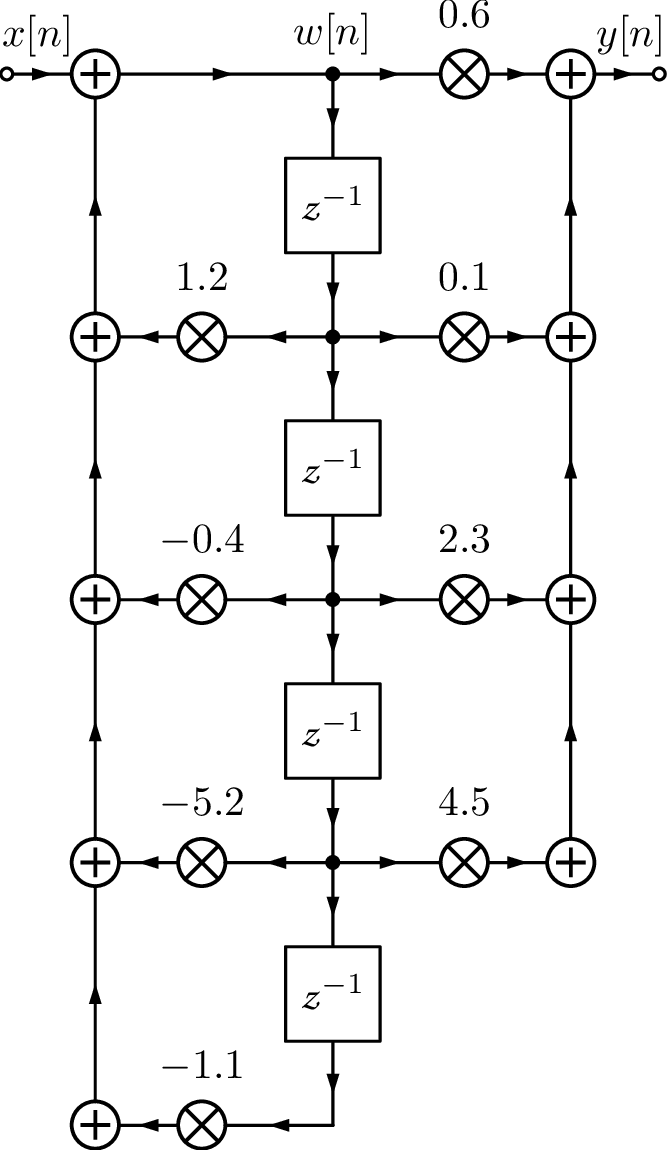
Figure 3.55(a) depicts the implementation of $H (z)$ using the direct form I structure. Note that 7 delay blocks were used, which corresponds to requiring 7 memory locations to store their outputs. In case each number is represented by 16 bits, this would require 14 bytes. It is possible to reduce this number to 8 bytes using a direct form II structure, as depicted in Figure 3.55(c).

The direct form II can be derived from the form I by noting that $H (z)$ is a LTI system and the following is valid:

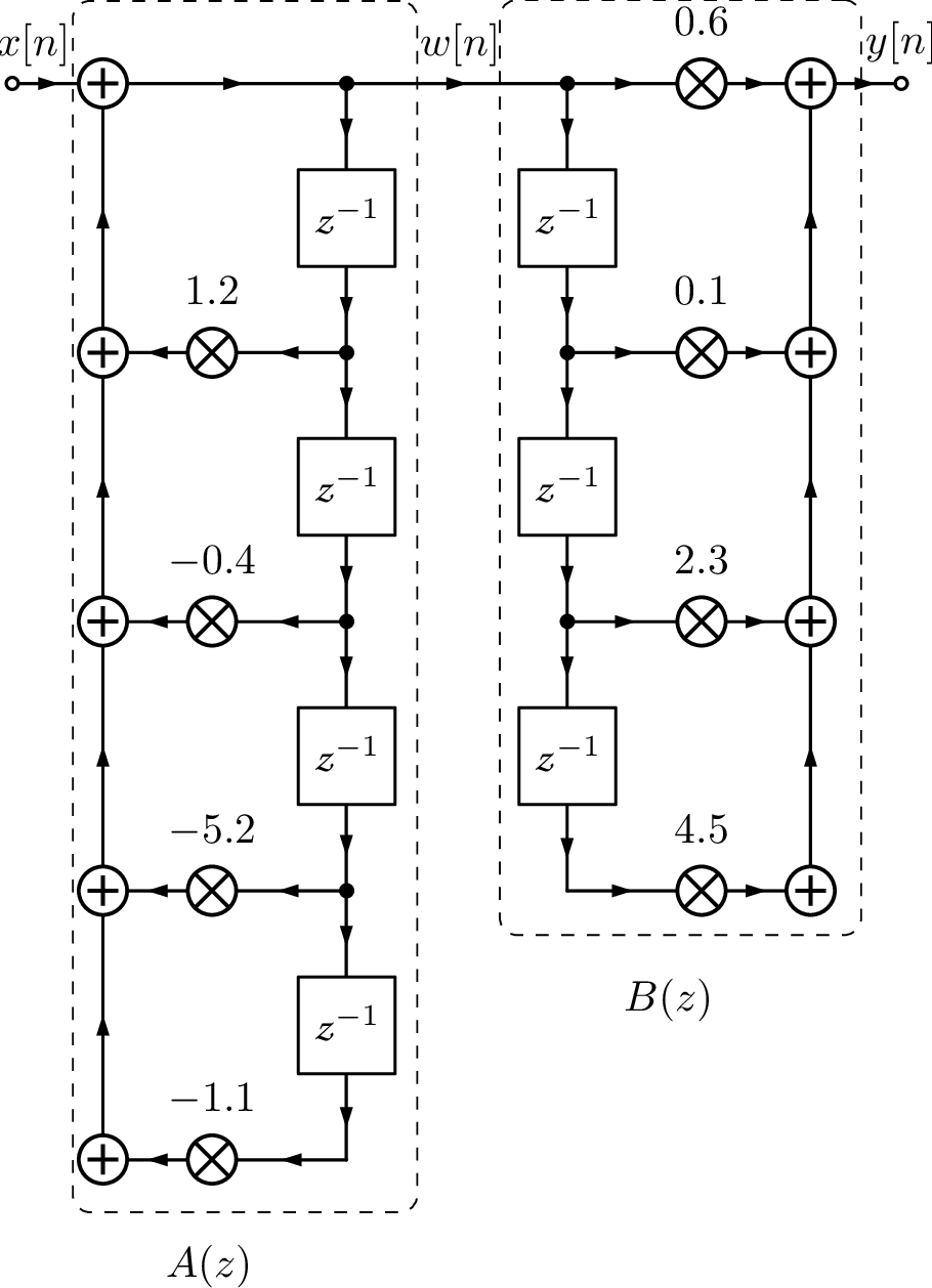
\begin{array}{l} x [n] \to B (z) \to z [n] \to A (z) \to y [n] \\ \equiv x [n] \to A (z) \to w [n] \to B (z) \to y [n] . \end{array}

However, there is a disadvantage in implementing the poles first, as done in the direct form II: the signal can saturate in intermediate stages of filtering. When using the direct form I, the zeros tend to attenuate the signal and, after this attenuation, the poles amplify some frequency components. The net result should be no overflows. On the other hand, the direct form II first amplifies via the poles and later attenuates via the zeros. To circumvent this disadvantage while retaining the property of requiring the minimum amount of delay blocks, the direct form II can be transposed. In other words, while the form I implements $B (z)$ first (corresponding to the zeros), the form II implements $A (z)$ first. This new order allows sharing the delay blocks and reduces their number to the order of the filter ( $M = 4$ in the example of Figure 3.55). Figure 3.55(b) shows the intermediate step when one goes from direct form I to II.

Figure 3.56: IIR of Eq. (3.97) implemented with the transposed direct form II. The intermediate diagram in (a) is obtained by transposing Figure 3.55(c), while (b) simply reorganizes it.

The transposed direct form II is based on the fact that with three steps: a) inverting the orientation of all “arrows” in signal flow graph, b) swapping input $x [n]$ and output $y [n]$ , and c) swapping adders by signal “splitters” and vice-versa, one obtains a structure that implements the same difference equation of the original structure.

If the IIR filter has order $M > 2$ it is common to organize its poles and zeros as second order sections (SOS). For example, a filter $H (z)$ of order $M = 7$ can be implemented as a cascade connection $H (z) = H_{1} (z) H_{2} (z) H_{3} (z) H_{4} (z)$ of three SOS $H_{1} (z), H_{2} (z), H_{3} (z)$ and one first-order section $H_{4} (z)$ as indicated by:

\begin{array}{l} x [n] \to H (z) \to y [n] \\ \equiv x [n] \to H_{1} (z) H_{2} (z) \to H_{3} (z) \to H_{4} (z) \to y [n] . \end{array}

It is also possible to decompose $H (z)$ into SOS sections that are organized in parallel, such that $H (z) = G_{1} (z) + G_{2} (z) + G_{3} (z) + G_{4} (z)$ for this example, with $G_{4} (z)$ being a first-order section. The commands residue and residuez are helpful to obtain the partial fractions expansion in the Laplace and Z transform domains, respectively, and are useful when designing the parallel structure. Using residuez and assuming that $H (z)$ is given by Eq. (3.97), one can find the parallel structure with the commands:

Listing 3.32: MatlabOctaveCodeSnippets/snip_systems_residuez.m

1b=[0.6 0.1 2.3 4.5]; 
2a=[1 -1.2 0.4 5.2 1.1]; 
3[r,p,k]=residuez(b,a); %fraction expansion in Z domain 
4%note that using [b,a]=residuez(r,p,k) reconstructs b,a 
5%hence, create two SOS with pairs of fractions: 
6[b1,a1]=residuez([r(1) r(2)],[p(1) p(2)],0) 
7[b2,a2]=residuez([r(3) r(4)],[p(3) p(4)],0)

The hint is that residuez can be used for decomposing in fractions and also for organizing pairs of fractions as second-order sections. The last two commands in the previous code reorganizes pairs of fractions, i. e., it implements

\frac{r_{1}}{1 - p_{1} z^{- 1}} + \frac{r_{2}}{1 - p_{2} z^{- 1}} = \frac{r_{1} + r_{2} - (r_{1} p_{2} + r_{2} p_{1}) z^{- 1}}{(1 - p_{1} z^{- 1}) (1 - p_{2} z^{- 1})},

where $r_{i}$ is the residue of pole $p_{i}$ . Therefore, Eq. (3.97) can be written as

H (z) = \frac{- 0.1637 + 1.3542 z^{- 1}}{1 - 2.6669 z^{- 1} + 4.0399 z^{- 2}} + \frac{0.7637 + 1.0226 z^{- 1}}{1 + 1.4669 z^{- 1} + 0.2723 z^{- 2}} .

The cascade structure with each SOS implemented with a transposed direct form II can be considered the most popular realization and will be emphasized here.

Decomposing $H (z)$ in sections allows an easier control of issues provoked by using finite precision. For example, the poles with higher quality factor $Q$ can be placed last in the cascade and pairs of zeros “paired” (or “matched”) to pairs of poles to minimize the chances of signal saturation at intermediate stages.

Table 3.10: Matlab/Octave functions to convert among the formats: transfer function (tf), zero-pole (zp) and second order sections (sos). The number two is a mnemonic for “to”.

	tf	zp	sos
tf		tf2zp	tf2sos
zp	zp2tf		zp2sos
sos	sos2tf	sos2zp

Matlab/Octave offers several functions to deal with SOS, as indicated in Table 3.10. The description of $H (z)$ with $S$ sections uses a matrix of dimension $S \times 6$ , where each row describes a SOS

H_{s} (z) = \frac{b_{0} + b_{1} z^{- 1} + b_{2} z^{- 2}}{1.0 + a_{1} z^{- 1} + a_{2} z^{- 2}}

via a vector $[b_{0}, b_{1}, b_{2}, 1, a_{1}, a_{2}]$ . For example, Eq. (3.97) can be decomposed in SOS with:

Listing 3.33: MatlabOctaveCodeSnippets/snip_systems_SOS_decomposition.m. [ Python version]

1B=[0.6 0.1 2.3 4.5]; %numerator 
2A=[1 -1.2 0.4 5.2 1.1]; %denominator 
3[z,p,k]=tf2zp(B,A); %convert to zero-pole for improved 
4[sos,g] = zp2sos(z, p, k) %to SOS, g is the overall gain

The Octave implementation of the zp2sos function is slightly different from Matlab’s. The gain g=0.6 obtained with the previous commands is the same for both Matlab and Octave. But the sos matrix in Matlab is:

sos =    0    1.0000    1.3689    1.0000    1.4669    0.2723
    1.0000   -1.2022    5.4790    1.0000   -2.6669    4.0399

while in Octave it is:

sos = 1.00000  -1.20220   5.47898   1.00000  -2.66692   4.03987
      1.00000   1.36887  -0.00000   1.00000   1.46692   0.27229

The comparison shows that the order of SOS is inverted: by default Matlab orders the sections with poles closest to the unit circle (higher $Q$ ) last in the cascade while Octave performs the opposite. Another difference is the representation of the SOS with a numerator $(1 + 1.3689 z^{- 1})$ of order 1. The Matlab’s version is

H (z) = 0.6 (\frac{1 + 1.3689 z^{- 1}}{1 + 1.4669 z^{- 1} + 0.2723 z^{- 2}}) (\frac{1 - 1.2022 z^{- 1} + 5.4790 z^{- 2}}{1 - 2.6669 z^{- 1} + 4.0399 z^{- 2}}),

which is represented using transposed direct form II sections in Figure 3.57.

Figure 3.57: Realization of Eq. (3.97) with transposed direct form II second order sections.

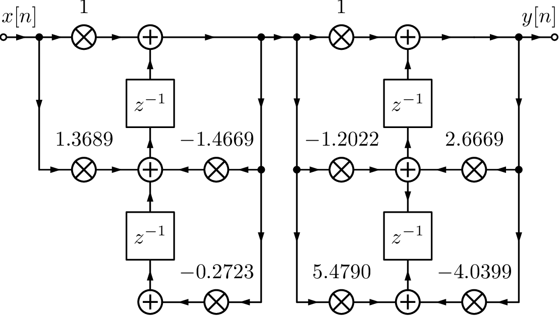
It is important to note that using zero/pole ( $[z, p, k]$ syntax) to design IIR filters is better than using transfer functions with respect to numerical accuracy. After obtaining $[z, p, k]$ , one can analyze or implement the filter using SOS (via zp2sos). For filters of order higher than 7, numerical problems may happen when forming the transfer function ( $[b, a]$ syntax).³⁷

3.15.3 Running a digital filter using filter or conv

Any LTI system $H (z)$ can be represented by an impulse response $h [n]$ . Having $h [n]$ , one can use convolution to obtain $y [n] = x [n] * h [n]$ . On a computer, it may be necessary to truncate an infinite duration $h [n]$ . Matlab/Octave has the function impz that, based on $H (z)$ , can obtain a vector h representing $h [n]$ . However, if $H (z) = B (z) ∕ A (z)$ represents a LCCDE, it is typically more efficient to implement an IIR via its difference equation with y=filter(B,A,x) than via convolution with y=conv(x,h). When comparing the result of these two options, it is important to note that conv outputs a vector of length $N_{y} = N_{x} + N_{h} - 1$ , where $N_{x}$ and $N_{h}$ are the lengths of x and h, respectively, while filter always has $N_{y} = N_{x}$ because it truncates the tail of the corresponding convolution.

3.15.4 Advanced: Effects of finite precision

When implementing a digital filter using finite precision there are two aspects to consider:

The quantization of the filter coefficients of $H (z)$ leads to another transfer function $H_{q} (z)$ with, eventually, displaced poles and zeros, frequency response, etc.
During runtime, the result of multiplications and additions are quantized and this error impacts the system output. This is called round-off or rounding error.

It is possible to implement digital filters using floating-point arithmetics. This is performed by Matlab/Octave, for example, which can operate with double precision (each number represented by 64 bits). This is considered the representation with infinite precision here. For the study of finite precision effects, it will be assumed a fixed-point representation.

Quantization of the filter coefficients via examples

This section briefly discusses the issue of quantizing the filter coefficients via examples. Recall from Section A.28.1 that $b_{i}$ and $b_{f}$ are the number of bits assigned to the integer and fractional part of the number, respectively.

In order to study the effect of coefficient quantization, a 8-th order bandpass filter was used. It was designed with the commands in Listing 3.34.

Listing 3.34: MatlabOctaveCodeSnippets/snip_systems_coefficient_quantization.m. [ Python version]

1Apass=5; %maximum ripple at passband (dB) 
2Astop=40; %minimum attenuation at stopband (dB) 
3Fs=500; % sampling frequency 
4Wr1=10/(Fs/2); %normalized frequencies (from 0 to 1): 
5Wp1=20/(Fs/2); %frequencies in Hz are divided by ... 
6Wp2=120/(Fs/2);%the Nyquist frequency Fs/2 
7Wr2=140/(Fs/2); 
8[N,Wp]=ellipord([Wp1 Wp2],[Wr1 Wr2],Apass,Astop) %order,Wp 
9[z,p,k]=ellip(N,Apass,Astop,Wp); %design digital filter 
10[B, A]=zp2tf(z,p,k); %zero-pole to transfer function

After the filter is designed, with its coefficients represented in double precision, Matlab or Octave can be used to find their fixed point representations.

Using Matlab, the coefficients of the filter can be quantized with the commands in Listing 3.35.

Listing 3.35: MatlabOnly/snip_systems_Matlab_coef_quant.m. [ Python version]

1bi=7; % number of bits for integer part 
2bf=8; % number of bits for decimal part 
3b=bi+bf+1; %total number of bits, inclusing sign bit 
4signed=1; %use signed numbers (i.e., not "unsigned") 
5Bq=fi(B,signed,b,bf); %quantize coefficients of B(z) using Q7.8 
6Aq=fi(A,signed,b,bf); %quantize coefficients of A(z) using Q7.8 
7zplane(double(Bq),double(Aq)) %cast to double before manipulating

Using Octave, the quantization code is Listing 3.36.

Listing 3.36: OctaveOnly/snip_systems_Octave_coef_quant.m. [ Python version]

1bi=7; % number of bits for integer part 
2bf=8; % number of bits for decimal part 
3Bq=fixed(bi,bf,B); %quantize coefficients of B(z) using Q7.8 
4Aq=fixed(bi,bf,A); %quantize coefficients of A(z) using Q7.8

Figure 3.58: The original magnitude response of the 8-th order filter and its 16-bits per coefficient Q7.8 quantized version ( $b_{i} = 7$ and $b_{f} = 8$ ).

Figure 3.59: Zeros and poles for the original and quantized filters discussed in Figure 3.58.

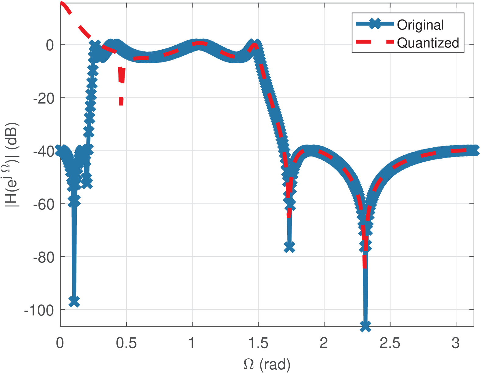
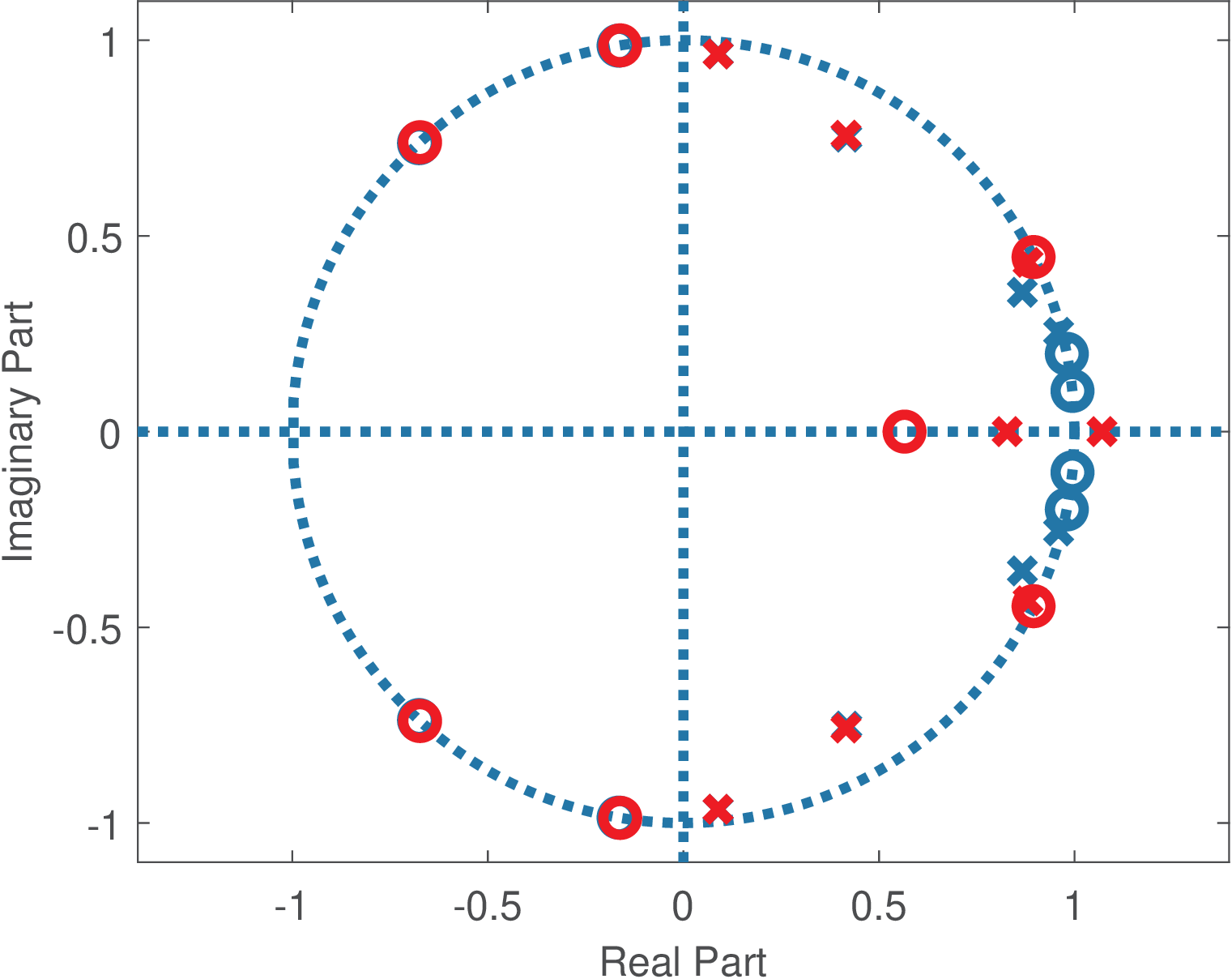
Figure 3.58 shows the magnitude responses of the original and quantized filters, and one can see that there is a discrepancy close to DC. Figure 3.59 shows zeros and poles for the same pair of filters. One can note that the pair of poles close to DC get transformed into real poles. This impacts the frequency response and creates the mentioned discrepancy.

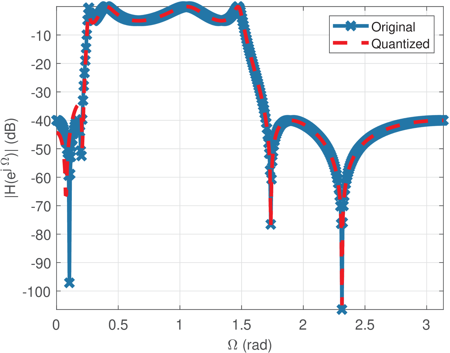
Figure 3.60: Magnitude of quantized filter with Q10.15 using 26 bits ( $b_{i} = 10$ and $b_{f} = 15$ ) and the original filter of order 8 in Figure 3.58.

Figure 3.60 is the result of increasing the number of bits to $b = 26$ , with $b_{i} = 10$ and $b_{f} = 15$ when quantizing the eighth-order filter. It can be observed that good results are obtained. However, $b = 26$ bits does not always guarantee good results. The following example illustrates that a good choice of $b$ depends on aspects such as the filter order.

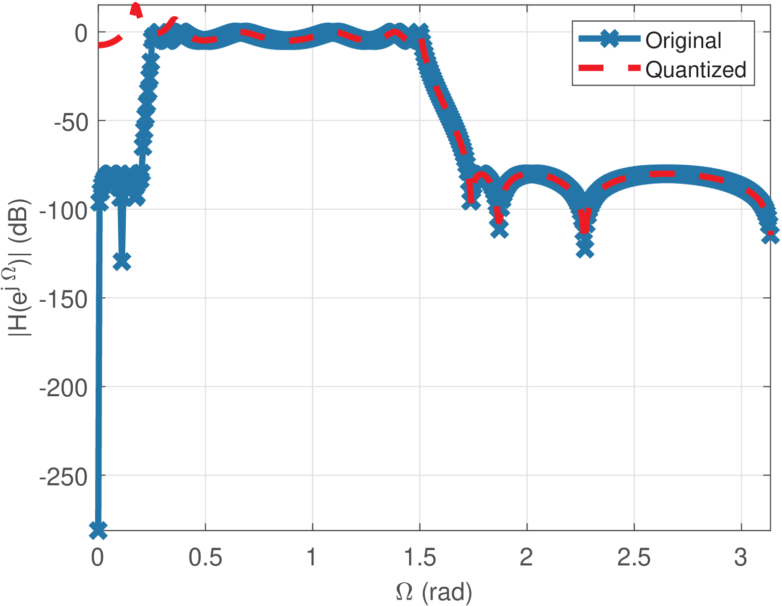
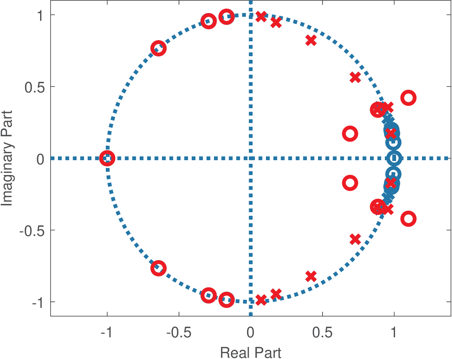
Figure 3.61: Magnitude responses for original filter of order 14 and its quantized version with $b = 26$ bits ( $b_{i} = 10$ and $b_{f} = 15$ ).

Figure 3.62: Zeros and poles for the corresponding filter in Figure 3.61. Note the occurrence of poles outside the unit circle, which make the quantized filter unstable.

Changing the filter mask of the original 8-th filter to impose Astop=80 increases the filter order from 8 to 14. Now, quantization with 26 bits generates an unstable filter as illustrated in Figure 3.61 and Figure 3.62.

Roundoff errors during the signal processing

The analysis of the quantization error created along the filtering process is more involved than observing the effect of filter coefficients quantization. Note that the term roundoff is used even when truncation is the actual operation, as done by Octave’s fixed point package.

When interested on evaluating the roundoff errors, it does not suffice to pass objects of the fixed point class (called FixedPoint and embedded.fi in Octave and Matlab, respectively) to a specific function. For example, considering filter, the internal operations within this function may not have its results quantized. To study the roundoff errors, one typically has to write a function that internally represents the numbers in fixed point too. Listing 3.37 and Listing 3.38 illustrate this point. Octave was adopted for the former code and Matlab for the latter. The commands for dealing with fixed point in both are discussed in Section A.28.1.

Listing 3.37: OctaveOnly/snip_systems_filtering_precision.m. [ Python version]

1N=100; %number of samples 
2x=20*randn(1,N); %gerante random samples 
3M=4; %filter order 
4[B,A]=butter(M,0.3); %design IIR filter 
5%Define fixed-point elements: 
6bi=3; % number of bits for integer part 
7bf=5; % number of bits for fractional part 
8xf=fixed(bi,bf,x); %quantize the input 
9Bf=fixed(bi,bf,B); %quantize the filter's numerator 
10Af=fixed(bi,bf,A); %quantize the filter's denominator 
11y1=filter(B,A,x); %output with ("infinite") double precision 
12y2=filter(Bf,Af,x); %quantized: only filter coefficients 
13y3=filter(Bf,Af,xf);%quantized: input and coeffficients 
14y4=filter(B,A,xf); %quantized: only input 
15y5=fixed(bi,bf,y1); %quantized: input, output and coefficients

Listing 3.37 uses filter and illustrates how the signals and coefficients can be quantized. When observing the signal y5, one may consider that all the processing used fixed point numbers in Q3.5 format. However, the internal variables used by filter were not quantized. In other words, internally, filter does not uses finite precision arithmetics. This is circumvented in Listing 3.38.

Listing 3.38: MatlabBookFigures/figs_systems_roundoffErrors

1function [yq_my, y_my, y_matlab]=figs_systems_roundoffErrors 
2N=30; %number of samples 
3x=7*randn(1,N); %generate N random samples 
4y=zeros(size(x)); %pre-allocate space for output 
5M=4; %filter order 
6[B,A]=butter(M,0.3); %design IIR filter 
7bi=2; % number of bits for integer part 
8bf=3; % number of bits for fractional part 
9b=bi+bf+1; %total number of bits, inclusing sign bit 
10signed=1; %use signed numbers (i.e., not "unsigned") 
11xf=fi(x,signed,b,bf); %create variables with fixed-point, input 
12yf=fi(y,signed,b,bf); %filter output 
13Bq=fi(B,signed,b,bf); %quantized B(z) coefficients 
14Aq=fi(A,signed,b,bf); %quantized A(z) coefficients 
15if sum(abs(Bq))==0 || sum(abs(Aq))==0 
16    error('Quantized filter has B(z) or A(z) only with zero values!') 
17end 
18%1) everything quantized: coeffs, input, internal processing: 
19zeroReference=fi(0,1,2*b,2*bf+1);%using to make acc a fixed-point obj 
20yq_my=myFilter(Bq,Aq,xf,yf,zeroReference); %all inputs in fixed-point 
21%2) no quantization, but using myFilter function: 
22zeroReference=0; %it is a double, so it will be the acc in myFilter 
23y_my=myFilter(B,A,x,y,zeroReference); %note that x,y,etc are double's 
24%3) no quantization, but using Matlab's filter: 
25y_matlab=filter(B,A,x); 
26end 
27function y = myFilter(Bq,Aq,xn,yn,zeroReference) 
28M=length(Bq)-1; %get the order of the filter's numerator ... 
29N=length(Aq)-1; %and denominator 
30%Note: this code does not treat the transient in first samples and 
31%will differ from Matlab's filter during the transient. 
32for n=N+1:length(xn) %after transient 
33    acc = zeroReference;%resets accumulator,assume fi(0,1,2*b,2*bf+1) 
34    for i=0:M %implement Direct-II Transposed as Matlab's filter 
35        acc = acc + Bq(i+1)*xn(n-i); %implements numerator 
36    end 
37    for i=1:N %Note, the code assumes A(1) = 1 
38        acc = acc - Aq(i+1)*yn(n-i);%implements denominator 
39    end 
40    yn(n) = acc; %update the output 
41end 
42y=yn; %make the output equal to yn (yn is double or fixed point) 
43end

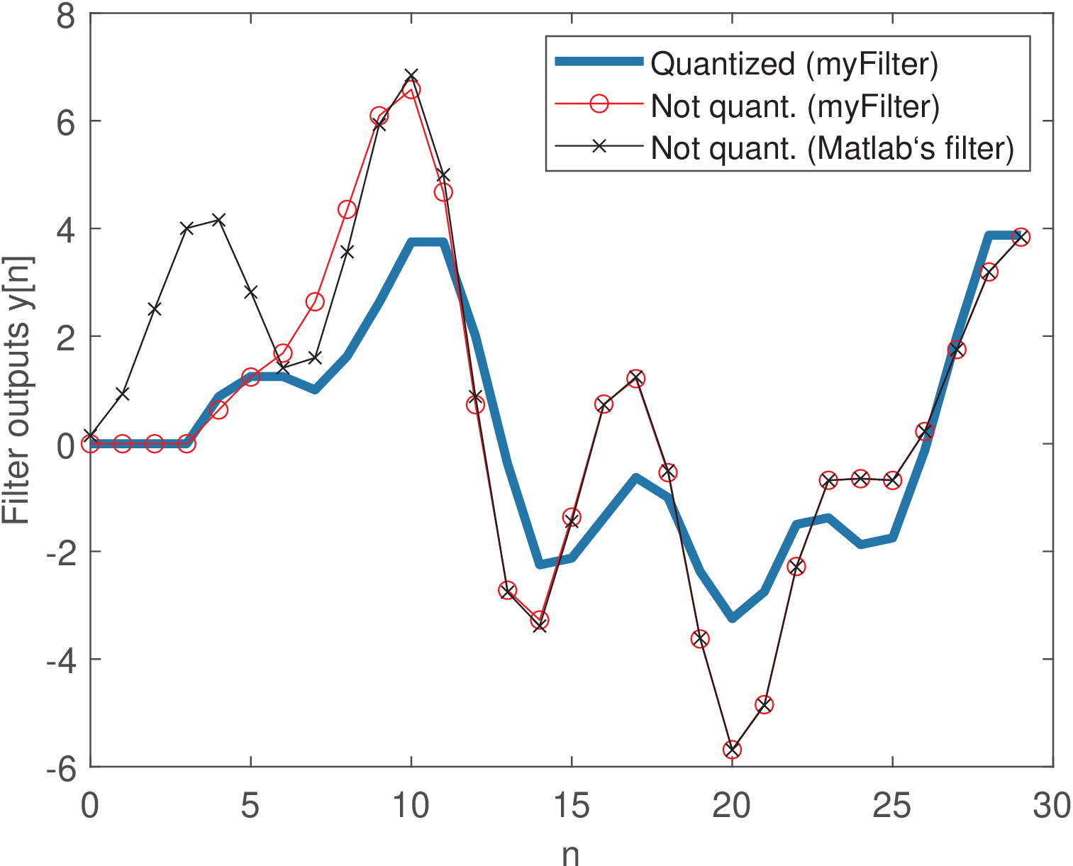
Figure 3.63: Example of filter outputs with floating-point double precision and fixed-point using Q2.3 generated with Listing 3.38.

Listing 3.38 was used to generate Figure 3.63 with three signals: one obtained with fixed-point processing and two other not-quantized signals, which were obtained with myFilter and Matlab’s filter for validation purposes. It can be seen that the non-quantized signals differ only during the transient part, as commented in the source code of myFilter. Other than that, the signals are equivalent.

Observe that myFilter provides support to using a special register called accumulator, which is typical in digital signal processor chips, and in this case uses twice the number of bits of the other registers. For example, when the regular registers have 16 bits, the accumulator may have 32 bits, to minimize the roundoff error. The number representation adopted during the internal processing within myFilter is determined by the type (or class) of the inputs passed to the function. In the first call to myFilter in Listing 3.38, the variable zeroReference and all others are fixed point objects and the function is careful to not change this condition. For example, using a command such as acc = 0 would make acc a “double” variable, not an object of the fixed point class anymore. In the second call, all myFilter inputs are in double precision and the result is equivalent to filter after the transient.

It can be seen from Figure 3.63 that the quantized output has restricted range due to the small number of bits assigned to the integer part according to the Q2.3 representation. The reader is invited to run the code with a larger value for bi and even modify it to properly deal with the transient in a Transposed Direct-II realization.

³⁶ Matlab’s fdatool, via its menu Edit, provides support to converting the structure and also to showing it.

³⁷ See Matlab’s documentation for the filter function for more details.