Advanced: Bandwidth and Quality Factor

3.7 Advanced: Bandwidth and Quality Factor

3.7.1 Bandwidth and Quality Factor of Poles

The overall behavior of a filter is dictated by the combined effect of its poles and zeros. The position of a pole in the $s$ or $Z$ plane determines how it influences the overall system function ( $H (s)$ or $H (z)$ , respectively).

It can be shown that asymptotically each pole contributes with a roll-off of 20 dB per decade (equivalent to 6 dB per octave) and a zero with an increase of 20 dB per decade. This asymptotic behavior is used to obtain graphs known as Bode diagrams. This clearly indicates that the sharpness of a frequency response (shorter transition regions) can be improved by increasing the order of the corresponding system function $H (s)$ (or $H (z)$ ), i. e., adding poles and/or zeros. However, increasing the order of an analog filter requires more components (capacitors, opamps, etc.) and for a digital filter it requires more multiplications and additions. Hence, it is important to make the best use of poles (and zeros) and, motivated by that, to have figures of merit for them.

Besides its frequency, the bandwidth and quality factor of a single pole or zero are important to assess its influence. Poles will be emphasized in this section, but similar definitions are applied to zeros. This section discusses characteristics of a single pole while Section 3.7.2 extends the definitions to filters.

Bandwidth of a pole

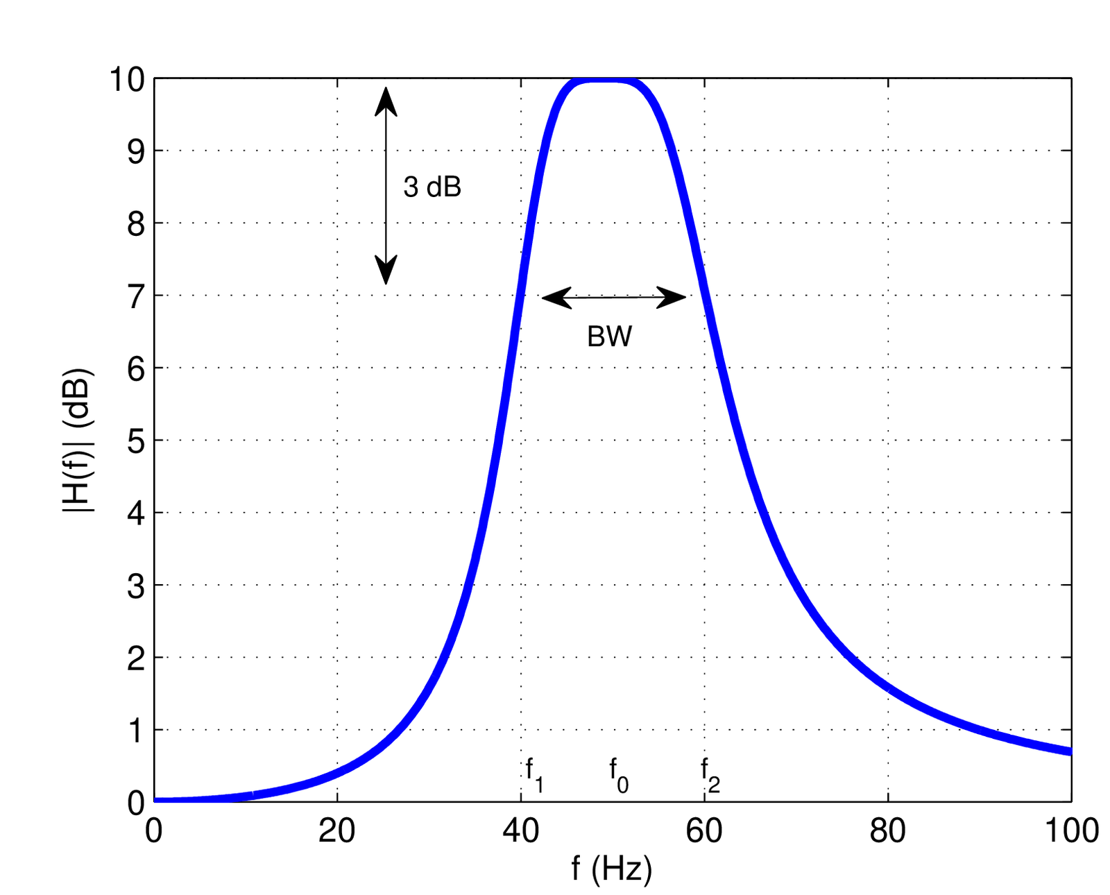
The bandwidth of a pole is illustrated in Figure 3.22 and defined here as $BW = f_{2} - f_{1}$ , where the cutoff frequencies $f_{1}$ and $f_{2}$ are those in which the gain $| H (f_{0}) |$ at the center frequency $f_{0}$ (that may be different than the natural frequency $f_{n}$ ) has decreased to $| H (f_{0}) | ∕ \sqrt{2}$ . The factor $1 ∕ \sqrt{2}$ corresponds to $20 {log}_{10} (1 ∕ \sqrt{2}) - 3.0103$ dB, or approximately $- 3$ dB. Therefore, this definition is called the 3-dB bandwidth or half-power BW.

Figure 3.22: Bandwidth $BW = f_{2} - f_{1}$ defined by the cutoff frequencies where the gain falls $- 3$ dB below the reference value at $f_{0}$ .

Pole bandwidth in continuous-time

Assuming a first-order system $H (s) = - α ∕ (s - p)$ , where $p = α + j ω_{0}$ is the pole, the bandwidth of $p$ in Hz is given by

BW = \frac{| α |}{π} .

(3.33)

This result can be obtained by noting that for any frequency $ω$

| H (ω) | = \frac{| α |}{\sqrt{{(ω - ω_{0})}^{2} + α^{2}}} .

Hence, the squared gain at the specific pole frequency $ω = ω_{0}$ is

| H (ω_{0}) |^{2} = \frac{α^{2}}{{(ω_{0} - ω_{0})}^{2} + α^{2}} = 1

and the squared gains at cutoff frequencies $ω = ω_{0} \pm α$ fall to $1 ∕ 2$ as required by the definition of cutoff frequency:

| H (ω_{0} \pm α) |^{2} = \frac{α^{2}}{{(ω_{0} \pm α - ω_{0})}^{2} + α^{2}} = \frac{1}{2} .

(3.34)

Hence, a range from $ω_{0} - α$ to $ω_{0} + α$ is determined by the two cutoff frequencies of a pole at $ω_{0}$ such that its bandwidth $BW$ is $2 | α |$ rad/s. Dividing by $2 π$ leads to $BW = 2 | α | ∕ (2 π)$ in Hz, as indicated in Eq. (3.33). A similar relation holds in discrete-time, as follows.

Pole bandwidth in discrete-time

Using the previous results and assuming the transformation $z = e^{s T_{s}}$ of Eq. (2.59), the pole $p = α + j ω_{0}$ in the plane $s$ is mapped into the pole $z = r e^{j Ω_{0}}$ in the plane $Z$ via

r e^{j Ω_{0}} = e^{p T_{s}} = e^{(α + j ω_{0}) T_{s}} = e^{α T_{s}} e^{j ω_{0} T_{s}} .

Hence, $r = e^{α T_{s}}$ and $Ω_{0} = ω_{0} T_{s}$ . Assuming $α < 0$ for a causal and stable $H (s)$ , Eq. (3.33) indicates that $α = - BW π$ , such that $r = e^{α T_{s}} = e^{- BW π T_{s}}$ and

BW = - \frac{ln (r)}{π T_{s}}

(3.35)

in Hz for a pole $r e^{j Ω_{0}}$ in the $Z$ plane with $r < 1$ .

One can rewrite Eq. (3.35) as $ln (r) = - BW π T_{s}$ and use the Taylor series expansion of $ln (\cdot)$ around a value $x = a$

ln (x) = ln (a) + \frac{1}{a} (x - a) - \frac{1}{2 a^{2}} {(x - a)}^{2} + \frac{1}{3 a^{3}} {(x - a)}^{3} - …,

with $a = 1$ , to keep only the first two terms and achieve

ln (r) \approx ln (1) + \frac{1}{1} (r - 1) = r - 1 .

Hence, the approximation $r - 1 \approx - BW π T_{s}$ allows to write

BW \approx \frac{(1 - r) F_{s}}{π},

(3.36)

which can be used when $r$ is close to 1.

Quality factor of poles

Besides the number of poles and zeros, another factor that influences the sharpness of a frequency response is the quality factor (or $Q$ -factor) of each pole, which is defined as

Q \overset{def}{=} \frac{f_{n}}{BW},

(3.37)

where $f_{n} = ω_{n} ∕ (2 π)$ is the natural frequency in Hz and $BW = f_{2} - f_{1}$ is the 3-dB bandwidth (also in Hz), as indicated in Figure 3.22.

For a second-order resonator, such as Eq. (3.27), the quality factor can be shown [ url3dsp] to be

Q = \frac{ω_{n}}{2 α} .

(3.38)

Appplication 3.3 presents a discussion on the influence of the Q-factor in frequency responses.

3.7.2 Bandwidth and Quality Factor of Filters

The previous definitions of bandwidth and Q-factor of poles can be extended to systems, especially frequency-selective filters such as bandpass and lowpass.

Bandwidth definitions for signals and systems

For a generic system there are definitions for the bandwidth ( $BW$ ) other than the 3-dB bandwidth of Figure 3.22. In all cases, if the frequency response has Hermitian symmetry, only the positive frequencies are taken in account.

A generalization of BW is to adopt the $X$ -dB bandwidth where $X$ is the attenuation of interest, such as 1 dB.

Alternatively, the absolute bandwidth can be applied when the signal is bandlimited. It is simply defined as the frequency range in which the spectrum is non-zero. For example, $H (f) = rect (f)$ has $BW = 0.5$ . Note that in this case the 3-dB BW definition would not be appropriate.

Another alternative definition of $BW$ is the so-called null-to-null or zero-crossing BW. In the case of a lowpass spectrum, the BW is determined by the first null of $| H (ω) |$ (or $| H (Ω) |$ in discrete-time). For example, a frequency response given by the $H (f) = sinc (fT)$ of Eq. (A.54) has $BW = 1 ∕ T$ according to this definition. For a passband spectrum, the two neighbor nulls of the center frequency determine BW. For example, the BW of $H (f) = sinc (fT - 5 T)$ is $BW = 2 ∕ T$ .

When a signal is complex-valued, its spectrum $X (f)$ does not have to exhibit Hermitian symmetry. In this case, the sampling theorem and other results depend on the double-sided or bilateral bandwidth, which takes in account the support of $X (f)$ from negative to positive frequencies.

For example, first consider the “conventional” case of $X (f)$ corresponding to a real-valued ideal lowpass filter with unitary gain from $- 200$ to 200 Hz: its BW is 200 Hz, and its double-sided bandwidth is 400 Hz. Contrast now with a complex-valued signal with $X (f)$ being a square pulse from $- 300$ to 100 Hz as depicted in Figure 3.14. In the latter case, the double-sided bandwidth continues to be 400 Hz but the conventional BW fails to indicate, for example, the minimum $F_{s}$ according to the sampling theorem. In this case, the sampling theorem could be stated with respect to the double-sided bandwidth.

Another approach when dealing with complex-valued signals is to assume that $X (f)$ is zero for negative frequencies (such signals are called “analytic”). In this case, the bandwidth BW takes in account only positive frequencies, as usual, but it may be misleading the fact that the sampling theorem in this case of an analytic signal can be stated as

F_{s} > BW .

(3.39)

For example, if $X (f)$ is non-zero from DC to 300 Hz, sampling the corresponding complex-valued (analytic) time-domain signal $x (t)$ at $F_{s} = 350$ Hz suffices to avoid aliasing. In this case, the first spectrum replica at positive frequencies has support from 0 to 300 Hz, the second one from 350 to 650 Hz, and so on, indicating that there is no aliasing.

A bandwidth definition very useful when dealing with filtered white noise is the equivalent noise bandwidth (ENBW). The ENBW of a filter $H (f)$ is the bandwidth of a fictitious ideal (e. g., lowpass or bandpass) filter $H_{e} (f)$ with rectangular spectrum that obeys

\int_{- \infty}^{\infty} | H (f) |^{2} d f = \int_{- \infty}^{\infty} | H_{e} (f) |^{2} d f

(3.40)

and has the maximum value $H_{max}$ of $| H_{e} (f) |$ is equal to the maximum of $| H (f) |$ . The name ENBW is because both filters lead to the same output power when the input is white noise (discussed in details later, in Section 4.5.2 ) such that the equivalent filter can substitute the original (and more complicated one) while leading, for instance, to the same SNR in a simulation or theoretical development.

An example is provided in Figure 3.23, which was obtained with Matlab’s function⁹ enbw as informed in Listing 3.9. In this case, the ENBW was $102.4 ∕ 50 \approx 2$ times larger than the cutoff frequency.

Listing 3.9: Code/MatlabBookFigures/figs_digicomm_enbw

1Fs = 1000; %sampling frequency in Hz 
2fc = 50; %filter cutoff frequency in Hz 
3[B,A]=butter(4,fc/(Fs/2)); %4-th order Butterworth filter 
4N=100; %number of samples in impulse response hn 
5hn = impz(B,A,100); %impulse response 
6Hf = fftshift(fft(hn)); %sampled DTFT 
7equivalentBW = enbw(hn,Fs); %estimate equivalent noise bandwidth 
8%code to plot the figure continues from here...

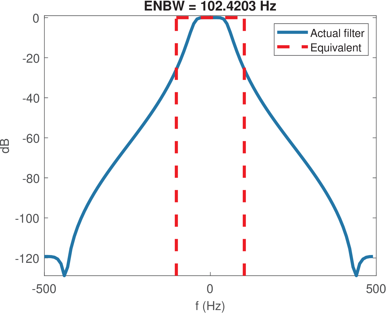
Figure 3.23: DTFT magnitude in dB of a 4-th order Butterworth filter with cutoff frequency of 50 Hz and the equivalent ideal filter with absolute bandwidth of 102.4 Hz.

Observing Figure 3.23, due to the rectangular shape of $| H_{e} (f) |$ ,

\int_{- \infty}^{\infty} | H_{e} (f) |^{2} d f = 2 ENBW \times H_{max}^{2} .

Hence, using Eq. (3.40) this can be written as:

ENBW = \frac{\int_{- \infty}^{\infty} | H (f) |^{2} d f}{2 H_{max}^{2}},

(3.41)

which for real signals simplify to

ENBW = \frac{\int_{0}^{\infty} | H (f) |^{2} d f}{H_{max}^{2}} .

(3.42)

Quality factor for filters

The Q-factor of a pole, as defined in Eq. (3.37), can be easily adapted to a system with a frequency response that allows obtaining its 3-dB bandwidth $BW$ (see Figure 3.22) such as a bandpass filter.¹⁰ In this case, the pole natural frequency $f_{n}$ in Eq. (3.37) is substituted by the filter’s center frequency $f_{c}$ such that

Q \overset{def}{=} \frac{f_{c}}{BW} .

(3.43)

The inverse of $Q$ , i. e., $BW ∕ f_{c}$ is called fractional bandwidth and often specified in percentage.

⁹ The function enbw was designed for lowpass (windows) spectra with the maximum value at DC. It does not work for passband spectra.

¹⁰ Actually, the Q factor is used in several areas of engineering and physics.