System Design with Bilinear Transformation

3.13 System Design with Bilinear Transformation

This section discusses the design of system functions $H (z)$ using the bilinear transformation. While $H (s)$ and $F_{s}$ were assumed to be known in the previous section, here the focus is on design, even in case $H (s)$ is not provided.

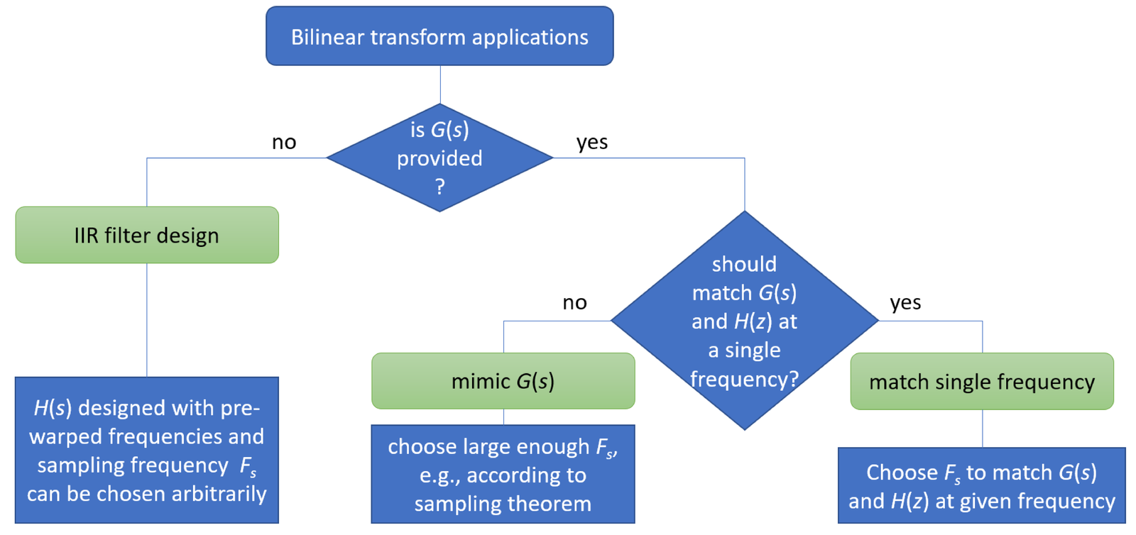
Figure 3.41: Three categories of bilinear applications and the respective choices of the sampling frequency $F_{s}$ in the bilinear transformation depends on the application, and can be arbitrary in the case of digital filter design.

The bilinear applications can be grouped in three main categories, as depicted in Figure 3.41:

Mimic $G (s)$ : A continuous-time system function $G (s)$ already exists and the goal is to find $H (z)$ (and $F_{s}$ ) that behaves, eventually in both time and frequency domains, as close as possible to $G (s)$ . In this case, the value of $F_{s}$ must be chosen according to the characteristics of the involved signals and impact the hardware (ADC, DAC and other components) used in the actual digital control system deployment. This is the case in some digital control applications. For instance, $G (s)$ may be a proportional-integral-derivative (PID) controller that needs to be converted to a discrete-time $H (z)$ and implemented in digital hardware (see, e. g., [ url3pid]). This category will be called here mimic $G (s)$ . We will denote the original system function as $G (s)$ to help distinguishing it from a continuous-time function $H (s)$ that is designed by the bilinear transformation user.
Match single frequency: In some applications, the goal is to use the bilinear transformation to find $H (z)$ that matches the behavior of a pre-existing continuous-time system function $G (s)$ at a single frequency. In this case, $G (s)$ may be a lowpass filter, for instance, and the matching frequency can be the cutoff frequency $ω_{c}$ of $G (s)$ . The bilinear sampling rate $F_{s}$ can be used to find $H (z)$ with the property of having a cutoff frequency $Ω_{c}$ that maps exactly at $ω_{c} = F_{s} Ω_{c}$ .
IIR filter design: This category concerns the design of IIR filters $H (z)$ with standard frequency responses: lowpass, highpass, bandpass and bandstop. In this case, even if the filter specification was given in continuous-time, it can be converted to a discrete-time specification. From this discrete-time specification, the designer can arbitrarily choose the value of $F_{s}$ to perform pre-warping, and then design $H (s)$ using well-known filter approximation methods such as Butterworth and Chebyshev. With $F_{s}$ and $H (s)$ , the discrete-time filter $H (z)$ is finally obtained through the bilinear transformation.

As highlighted in Figure 3.41, the designer can choose an arbitrary value for the sampling frequency $F_{s}$ when the bilinear is used to design a digital filter from a pre-warped continuous-time system function $H (s)$ . In contrast, in applications that fall within the mimic $G (s)$ category, $F_{s}$ should be carefully chosen. When the goal is use the bilinear to match a single frequency, a specific value of the sampling frequency can be used to define the matching frequency.

The next three subsections will discuss each of the categories in Figure 3.41.

3.13.1 Bilinear for IIR filter design

The design of IIR filters using the bilinear transformation relies on first designing an analog filter $H (s)$ using a classic approximation method. The most used methods are listed in Table 3.7. In applications in which the phase linearity is important, good options are the Bessel and Butterworth. However, their magnitude response does not represent a magnitude roll-off as steep as the other options. If the phase does not need to be approximately linear, Cauer (or elliptic) filters achieve a sharper roll-off and, consequently, a lower filter order for a given project specification. However, Cauer and Chebyshev Type I present ripple along the passband frequencies, which may be a problem in some applications. When compared to Chebyshev Type I, the Chebyshev Type II approximation has the advantage of having ripple only in the stopband.

Table 3.7: Main approximations adopted in the design of continuous-time filters

H (s)

with their pros and cons with respect to phase and magnitude (mag.).

Approximation	Pros	Cons
Bessel	Phase linearity	smooth (poor) mag. roll-off
Butterworth	Flat passband mag.	gradual (poor) mag. roll-off
Chebyshev Type I	Steeper mag. roll-off	ripple in passband
Chebyshev Type II	Steeper mag. roll-off	ripple only in stopband
Cauer (or elliptic)	Sharp (good) mag. roll-off	Non-linear phase and ripples

This subsection assumes the goal is to design an IIR filter $H (z)$ by applying the bilinear transformation to the designed $H (s)$ . The next paragraphs will emphasize the importance of pre-warping frequencies and finding the order of the analog filter $H (s)$ that complies with the project requirements.

In IIR filter design, there is no concern about the value of the sampling frequency. In this case, before obtaining the $H (s)$ that will be adopted for the bilinear transformation, it is important to pre-warp all frequencies of interest using Eq. (3.75). This way, the non-linear behavior imposed by the bilinear transformation (see, e. g. Figure 3.36 and Figure 3.35) is pre-compensated by the filter designer.

A key message is:

When designing a filter using the bilinear transformation, all frequencies of interest must be pre-warped and the design of $H (s)$ based on these modified frequencies. When $H (z)$ is obtained, the bilinear transform will “undo” the pre-warping and locate the frequencies in the desired positions.

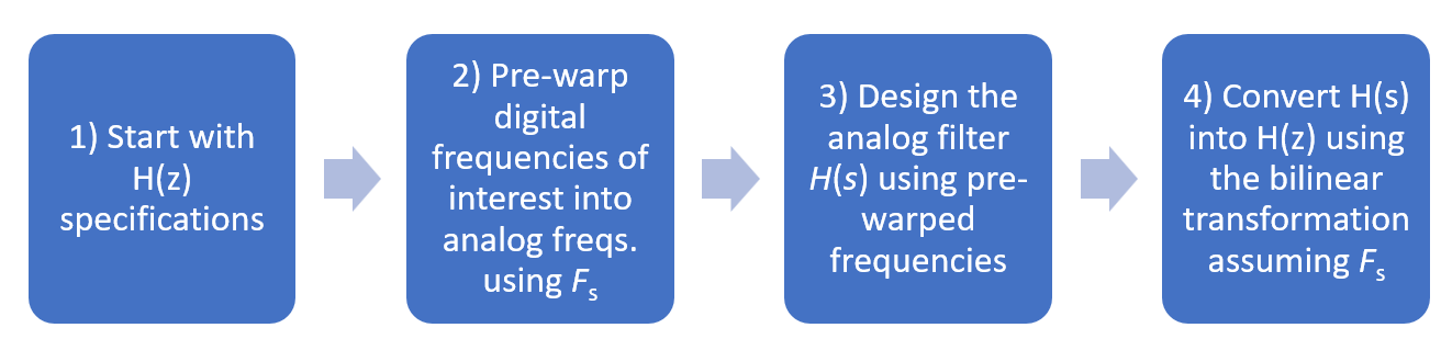
Figure 3.42 summarizes the steps when using the bilinear transformation for IIR design. Note that the value of the sampling rate $F_{s}$ is chosen in Step 2 and reused in Step 4, which then cancels out the influence of $F_{s}$ . This will be discussed later, after some examples of IIR design with bilinear.

Figure 3.42: Steps of IIR filter design using the bilinear transformation when the filter requirements are in discrete-time (frequencies in radians).

The following two examples illustrate pre-warping and finding the minimum order of a filter that complies with the project requirements. These projects use the bilinear function for pedagogical reasons. But instead of using this function, one could directly design IIR filters using higher-lever functions such as butter, cheby2 and others, which automatically invoke a bilinear routine.

Example 3.28. Design a digital lowpass filter using the bilinear transformation. The task is to design a Butterworth lowpass digital filter $H_{z} (z)$ with passband $Ω_{p} = π ∕ 5$ and stopband $Ω_{s} = 3 π ∕ 10$ frequencies, respectively, both in rad. Note that the specifications are in discrete-time. The maximum and minimum attenuations in pass and stopbands are $A_{p} = 4$ dB and $A_{s} = 10$ dB, respectively.

In order to use classic methods for designing analog filter $H (s)$ , the discrete-time frequencies $Ω_{p}$ and $Ω_{s}$ are converted to continuous-time assuming an arbitrary sampling frequency. Here we will assume $F'_{s} = 0.5$ Hz for convenience. Hence, using Eq. (3.75) the frequencies of interest are pre-warped to $ω_{p} = tan (Ω_{p} ∕ 2) \approx 0.325$ and $ω_{s} = tan (Ω_{r} ∕ 2) \approx 0.509$ rad/s.

To find the minimum order of a Butterworth that obeys the requirements, one can use:

1Ap=4; % maximum attenuation in passband (in dB) 
2As=10; % minimum attenuation in stopband (in dB) 
3wp=0.325; % passband frequency in rad/s 
4ws=0.509; % stopband frequency in rad/s 
5[n,w_cutoff] = buttord(wp,ws,Ap,As,'s') 
6[Bs,As]=butter(n,w_cutoff,'s')

The second-order Butterworth with 3-dB cutoff frequency of 0.294 rad/s obeys the corresponding mask and has the system function $H_{s} (s) = 0.086 ∕ (s^{2} + 0.416 s + 0.086)$ . In Python,²⁹ the commands are:

1import scipy.signal 
2Ap=4; # maximum attenuation in passband (in dB) 
3As=10; # minimum attenuation in stopband (in dB) 
4wp=0.325; # passband frequency in rad/s 
5ws=0.509; # stopband frequency in rad/s 
6[n,w_cutoff] = scipy.signal.buttord(wp ,ws ,Ap ,As ,analog=True) 
7[Bs, As]= scipy.signal.butter(n, w_cutoff, analog=True)

Note that, while Matlab/Octave identifies a continuous-time system with ’s’, Python uses analog=True.

Having obtained $H_{s} (s)$ , using Eq. (3.64) with $F'_{s} = 0.5$ Hz leads to

\begin{array}{l} H (z) & = \frac{0.086}{{(\frac{z - 1}{z + 1})}^{2} + 0.416 (\frac{z - 1}{z + 1}) + 0.086} \\ = \frac{0.086 {(z + 1)}^{2}}{{(z - 1)}^{2} + 0.416 (z - 1) (z + 1) + 0.086 {(z + 1)}^{2}} \\ \approx \frac{0.0575 + 0.1150 z^{- 1} + 0.0575 z^{- 2}}{1 - 1.2166 z^{- 1} + 0.4466 z^{- 2}} . \end{array}

The frequency response of the designed $H (z)$ has magnitudes $10 {log}_{10} | H_{z} (e^{j Ω_{p}}) |^{2} = - 3.96$ and $10 {log}_{10} | H_{z} (e^{j Ω_{r}}) |^{2} = - 10$ dB, which obey the requirements. Note that there is some slack at $Ω_{p}$ while the filter matches exactly³⁰ the requirement at $Ω_{s}$ . $□$

Example 3.29. Design a digital bandpass filter using the bilinear transformation. The goal is to design a filter with a bandpass from $0.2 π$ to $0.4 π$ rad, and stopbands from 0 to $0.1 π$ and from $0.5 π$ to $π$ rad. The filter must have less than 3 dB of ripple in the passband and at least 30 dB of attenuation in the stopbands. In this example, we will adopt $F'_{s} = 0.5$ Hz (an arbitrary value) and the Chebyshev Type II approximation, which does not have the ripples at the passband that Chebyshev Type I has.

Listing 3.25 indicates how to perform this filter design using Matlab/Octave.

Listing 3.25: MatlabOctaveCodeSnippets/snip_systems_iir_bilinear.m

1%% Passband specifications given in discrete-time: 
2Wp = pi*[0.2 0.4];   % Passband Frequencies (rad) 
3Wr = pi*[0.1 0.5];     % Stopband (rejection) Frequencies (rad) 
4Apass = 3;           % Maximum passband attenuation (ripple) (dB) 
5Astop = 30;          % Minimum stopband attenuation (dB) 
6%% Choose convenient sampling frequency 
7Fs=0.5; % in Hertz 
8%% Map from discrete to continuous-time using pre-warping 
9wp=2*Fs*tan(Wp/2); % in rad/s 
10wr=2*Fs*tan(Wr/2); % in rad/s 
11%% Design analog filter (use 's' to impose continuous-time) 
12[N,w_design] = cheb2ord(wp,wr,Apass,Astop,'s')%find the filter order 
13[Bs,As]=cheby2(N,Astop,w_design,'bandpass','s') %obtain H(s) = Bs/As 
14figure(1), freqs(Bs,As) %plot the frequency response of H(s) 
15%% Convert to discrete-time using bilinear 
16[Bz,Az]=bilinear(Bs,As,Fs) %obtain H(z) from H(s) with given Fs 
17%% Check some results: 
18figure(2), freqz(Bz,Az) %plot DTFT of H(z). Check values at Wp and Wr 
19s=1j*wp; Hs_at_wp=20*log10(abs(polyval(Bs,s)/polyval(As,s)))%cutoff 
20z=exp(1j*Wp); H_at_Wp=20*log10(abs(polyval(Bz,z)/polyval(Az,z))) 
21z=exp(1j*Wr); H_at_Wr=20*log10(abs(polyval(Bz,z)/polyval(Az,z)))

In case the sampling frequency $F'_{s}$ is changed (line Fs=0.5) in Listing 3.25, one can observe that this does not alter the final filter $H (z)$ given by [Bz, Az]. $□$

Bilinear sampling rate is arbitrary in IIR filter design

Example 3.26 shows the strong impact that $F_{s}$ may have when the bilinear transformation is applied to a given continuous-time system $H (s)$ . However, when using the bilinear in the specific task of designing a digital filter, the chosen value for $F_{s}$ will cancel out and have no influence on the design. This was mentioned in Figure 3.41 and can be experimentally observed by changing $F'_{s}$ in Example 3.28 or in Listing 3.25. This fact is demonstrated here through the design of a simple first-order digital filter $H (z)$ with cutoff frequency $Ω_{c}$ .

The following code uses symbolic math to obtain $H (s)$ after pre-warping and, then using bilinear to obtain $H (z)$ .

1%define s, z, natural frequency, damping ratio and sampling interval 
2syms Wc wc b0 a0 s z Fs %all as symbolic variables 
3%1) Filter requirements: 1st-order Butterworth, cutoff freq. Wc rad 
4%2) pre-warping 
5wc = 2*Fs*tan(Wc/2); 
6%3) Design H(s) with pre-warped frequencies. A first-order 
7% Butterworth with cutoff frequency of 1 rad/s is H(s)=1/(s+1). 
8Hs_prototype = 1/(s+1); 
9% Use frequency scaling s=s/wc to move the cutoff from 1 to wc rad/s 
10Hs=subs(Hs_prototype,s,s/wc); % Continuous-time H(s). 
11pretty(Hs) % Use pretty(Hs) to see it 
12%4) Bilinear transformation 
13Hz=subs(Hs,s,(2*Fs)*((z-1)/(z+1))); %bilinear: s <- 2/Ts*(z-1)/(z+1) 
14Hz=simplify(Hz); %simplify the expression 
15disp('H(z) obtained with the bilinear transform:') 
16pretty(Hz) %show it using an alternative view

We want to show that the value of the sampling rate $F'_{s}$ can be chosen arbitrarily in this IIR design. There is only one frequency of interest in this case to be pre-warped, which leads to $ω_{c} = 2 F'_{s} tan (Ω_{c} ∕ 2)$ . Starting with the first-order Butterworth prototype $H_{p} (s) = 1 ∕ (s + 1)$ with cutoff frequency equals to 1 rad/s, one uses frequency scaling to move the cutoff frequency to the pre-warped frequency $ω_{c}$ . Hence, after Step 3 of the code (which implements Step 3 of Figure 3.42), one has:

H (s) = H_{p} (\frac{s}{ω_{c}}) = \frac{1}{\frac{s}{ω_{c}} + 1} = \frac{1}{\frac{s}{2 F'_{s} tan (Ω_{c} ∕ 2)} + 1} .

After the bilinear transformation in Step 4, the code outputs:

H (z) = H (s) |_{s = 2 F_{s} \frac{z - 1}{z + 1}} = \frac{1}{\frac{z - 1}{tan (Ω_{c} ∕ 2) (z + 1)} + 1} .

One can observe that $H (z)$ does not depend on $F'_{s}$ because the value of $F'_{s}$ was canceled. This also happens for filters of order larger than 1.

Example 3.30. Another example of the arbitrary $F'_{s}$ getting canceled out. Assume a second-order digital lowpass filter $H (s) = 1 ∕ (s^{2} + \sqrt{2} s + 1)$ (a normalized Butterworth) meets the requirements in continuous-time. We want to use the bilinear transformation to obtain $H (z)$ with a 3-dB cutoff frequency of $π ∕ 4$ rad.

We can choose any convenient value for $F'_{s}$ and to illustrate that, instead of using a specific numeric value, the development will be made for a generic $F'_{s}$ .

Eq. (3.75) is adopted to perform pre-warping, which leads to

ω_{c} = 2 F'_{s} tan (\frac{π ∕ 4}{2}) \approx 0.8284 F'_{s} .

Then, Eq. (3.55) is used to perform frequency scaling and move the cutoff frequency $ω_{c} = 1$ rad/s of the prototype filter to $ω_{c} = 0.8284 F'_{s}$ . Substituting $s$ by $s ∕ ω_{c} = s ∕ (0.8284 F'_{s})$ leads to

H (s) = \frac{1}{{(\frac{s}{0.8284 F'_{s}})}^{2} + \sqrt{2} (\frac{s}{0.8284 F'_{s}}) + 1}

Now, the bilinear can be applied to $H (s)$ , which leads to

H (z) = H (s) |_{s = (2 F'_{s} \frac{z - 1}{z + 1})} = \frac{0.0976 z^{2} + 0.1953 z + 0.0976}{z^{2} - 0.9428 z + 0.3333} .

Note that $F'_{s}$ was canceled out because it only appeared in $H (s)$ dividing $s$ , which is later substituted by $2 F'_{s} \frac{z - 1}{z + 1}$ . $□$

In conclusion, the $F'_{s}$ value adopted for the bilinear can be different from the one actually used when implementing the digital filter $H (z)$ (for instance, in an embedded system with ADC and DAC chips). We will use $F'_{s}$ to denote the value used in the bilinear transformation and reserve $F_{s}$ to the adopted sampling frequency when implementing $H (z)$ , as depicted in Figure 3.43.

Figure 3.43: Version of Figure 1.45 and Figure 3.34 that considers both the bilinear transformation and the conversion of continuous to discrete-time via $ω = Ω F_{s}$ .

Hence, in this very specific application of bilinear, the sampling frequency $F'_{s}$ can be chosen arbitrarily. This may sound confusing³¹ because, as discussed here, there are other applications of the bilinear transformation in which the value of $F_{s}$ must be carefully chosen. In IIR design, one just needs to avoid choosing a too small value for $F'_{s}$ , which could eventually lead to numerical issues in the design of $H (s)$ due to an extreme pre-warping of frequencies of interest. Hence, for convenience, $F'_{s}$ is chosen to be 0.5, 1 or 2 Hz in IIR design.

Figure 3.43 takes in account that two sampling frequencies can be used in a bilinear transformation: $F'_{s}$ and $F_{s}$ . The former is used in the transform itself while the latter is adopted for the actual implementation of $H (z)$ in a filtering hardware such as the one depicted in Figure 3.30.

Example 3.31. Design an IIR filter with the bilinear transformation using frequency scaling of an analog prototype filter. The task is to design on Matlab (Octave has a slightly different syntax) a third-order lowpass Butterworth digital filter $H (z)$ using the bilinear transformation of $H_{p} (s) = 1 ∕ (s^{3} + 2 s^{2} + 2 s + 1)$ (that can be obtained with [Bs,As]=butter(3,1,’s’)), which has a cutoff frequency $ω_{c} = 1$ rad/s. Other project requirements are a sampling frequency of $F_{s} = 500$ Hz and $H (z)$ with a cutoff frequency $f_{d} = 100$ Hz (i. e., $ω_{d} = 2 π f_{d} \approx 628.3$ rad/s).

Pre-warping must be used because $ω_{c} = 1$ rad/s is the cutoff frequency of the prototype $H_{p} (s)$ that has to be mapped to $f_{d} = 100$ Hz when $H (z)$ is implemented.

We will arbitrarily adopt $F'_{s} = F_{s} = 500$ Hz. The goal is to find the frequency $ω_{a}$ to which $ω_{d} = 2 π f_{d}$ is mapped to. Eq. (3.77) leads to

ω_{a} = 2 F_{s} tan (\frac{ω_{d}}{2 F_{s}}) = 2 \times 500 tan (\frac{2 π 100}{2 \times 500}) \approx 726.52 rad/s,

which corresponds to $115.63$ Hz.

Now, frequency scaling must be applied to $H_{p} (s)$ in order to move its cutoff frequency from $ω_{c} = 1$ to $ω_{a} = 726.52$ rad/s. Substituting $s \leftarrow s' ∕ 726.52$ in $H_{p} (s)$ leads to

H (s) = \frac{3.8348 \times 1 0^{8}}{s^{3} + 1.453 \times 1 0^{3} s^{2} + 1.0557 \times 1 0^{6} s + 3.8348 \times 1 0^{8}} .

Applying the bilinear to $H (s)$ with $F'_{s} = F_{s} = 500$ Hz leads to $H (z) = (0.0985 + 0.2956 z^{- 1} + 0.2956 z^{- 2} + 0.0985 z^{- 3}) ∕ (1 - 0.5773 z^{- 1} + 0.4218 z^{- 2} - 0.0563 z^{- 3})$ . Evaluating $| H (z) |$ at $z = e^{j Ω}$ , with $Ω = 2 π f_{d} ∕ F_{s}$ , one obtains $1 ∕ \sqrt{2}$ . This indicates that, due to the pre-warping, the bilinear positioned the cutoff of $H (z)$ at the desired value of 100 Hz.

The next paragraphs illustrate how a computer can be used to carry out the whole procedure. A first approach is to design an analog filter by first pre-warping the cutoff frequency and then use the bilinear:

1fs=500; %sampling frequency (Hz) 
2[Bs,As]=butter(3,2*pi*115.63,'s'); %analog filter 
3[Bz,Az]=bilinear(Bs,As,fs); %convert analog to digital 
4z=exp(1j*2*pi*100/500); abs(polyval(Bz,z)/polyval(Az,z))%check cutoff

The second and simpler approach (at least from the user’s perspective) is to directly use a routine that incorporates pre-warping and bilinear transformation, such as butter:

1Fs=500;fd=100; fnormalized=fd/(Fs/2); [B2,A2]=butter(3,fnormalized)

(recall that Matlab/Octave deals with digital filters using frequencies in Hertz normalized by the Nyquist frequency as informed in Table 1.5). A comparison would show that [Bz,Az] and [B2,A2] have approximately the same elements.

A third way of dealing with a software routine that directly designs a digital filter is to convert the specification to discrete-time. In this case, $Ω = ω_{d} ∕ F_{s} \approx 1.2566$ rad is the desired cutoff frequency and $H (z)$ can be obtained with:

1Fs=500;Wd=2*pi*100/Fs;[B3,A3]=butter(3,Wd/pi)

Note that in this and in the previous (second) approach, the function butter.m was not informed about $F_{s}$ . Consequently, when the pre-warping was done inside butter.m, it used an arbitrary value of $F'_{s}$ to pre-warp, then obtained $H (s)$ , and converted using bilinear with $F'_{s}$ , such that the value of $F'_{s}$ gets canceled out, as previously explained. $□$

Bilinear IIR design can start from continuous-time specifications

In previous IIR designs, the filter specification was provided in the discrete-time domain. However, the design of a digital filter may also start from specifications in the analog domain. Figure 3.44 summarizes a project flow that includes both options when designing a filter $H (z)$ using the bilinear transformation.

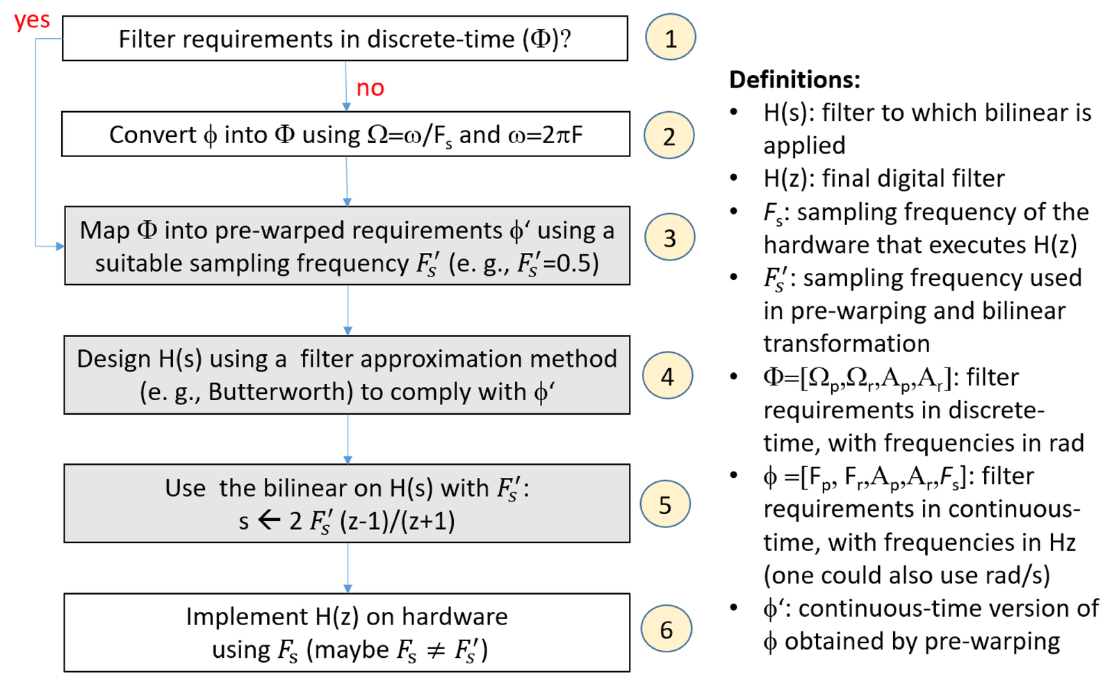
Figure 3.44: Steps for designing an IIR filter $H (z)$ using the bilinear transformation, assuming a lowpass filter. The set of requirements can be in discrete ( $Φ$ ) or continuous-time ( $ϕ$ ) domain.

Figure 3.44 considers the possibilities of having a set of filter requirements specified either in continuous ( $ϕ$ ) or discrete-time ( $Φ$ ). For example, a discrete-time lowpass filter can be specified by $Φ = {Ω_{p}, Ω_{r}, A_{p}, A_{r}}$ , where the subscripts $p$ and $r$ distinguish the frequencies and attenuations of the passband and stopband, respectively. Similarly, $ϕ = {F_{p}, F_{r}, A_{p}, A_{r}, F_{s}}$ is a possible lowpass filter requirement in continuous-time, as depicted in Figure 3.3(a). Note that $ϕ$ includes the sampling frequency $F_{s}$ used in the hardware implementation of the digital filter while $Φ$ does not.

In case the IIR design starts with filter requirements provided in discrete-time, $F_{s}$ is not part of the design process and $F'_{s}$ is chosen arbitrarily. The designer executes the steps “ $3 - 4 - 5$ ” depicted in Figure 3.44, as done in Example 3.28.

The next example illustrates a design using bilinear in which the specification $ϕ$ of the filter $H (z)$ to be designed is given in continuous-time, which includes the sampling frequency $F_{s}$ that will actually be used when implementing the filter.

Example 3.32. Bilinear design of IIR filter from continuous-time specifications. The task is to design an elliptic lowpass digital filter $H_{z} (z)$ that when implemented on a hardware operating at $F_{s} = 500$ Hz obeys the requirements $ϕ = {100, 150, 4, 20, 500}$ , where $ϕ = {F_{p}, F_{r}, A_{p}, A_{r}, F_{s}}$ with frequencies given in Hz.

According to Block 2 of Figure 3.44, using $ω = F_{s} Ω$ (Eq. (1.36)) and the definition of angular frequency $ω = F_{s} f$ , the continuous-time specifications $ϕ$ can be converted to the discrete-time specification $Φ = {0.4 π, 0.6 π, 4, 20}$ , where $Φ = {Ω_{p}, Ω_{r}, A_{p}, A_{r}}$ with frequencies given in radians. After this, one can continue to use $F_{s} = 500$ Hz or a new value for the sampling frequency can be chosen. For pedagogical purposes, a new value $F'_{s} = 0.5$ Hz is chosen here. Note that an important point is to use $F_{s} = 500$ Hz when implementing $H_{z} (z)$ on “hardware”, not $F'_{s}$ , which will be exclusively used for the design of $H (z)$ .

From Eq. (3.75) with $F'_{s} = 0.5$ , the frequencies of interest are pre-warped to $ω_{p} = tan (Ω_{p} ∕ 2) \approx 0.7265$ and $ω_{r} = tan (Ω_{r} ∕ 2) \approx 1.3764$ rad/s. Given the pre-warped specifications in continuous-time $ϕ' = {0.7265, 1.3764, 4, 20, 0.5}$ , one can obtain the second-order elliptic filter $H_{s} (s) = (0.1 s^{2} + 0.24) ∕ (s^{2} + 0.3542 s + 0.3803)$ that obeys the corresponding mask. This design of the analog filter $H_{s} (s)$ can be done with classical approximations and respective software, such as using ellipord and ellip in Matlab/Octave (see Listing 3.26).

Eq. (3.64) (with $F'_{s} = 0.5$ Hz) allows to convert $H_{s} (s)$ into $H_{z} (z) = (0.196 + 0.1614 z^{- 1} + 0.196 z^{- 2}) ∕ (1 - 0.7145 z^{- 1} + 0.5915 z^{- 2})$ , which has $10 {log}_{10} | H_{z} (e^{j Ω_{p}}) |^{2} = - 4$ and $10 {log}_{10} | H_{z} (e^{j Ω_{r}}) |^{2} = - 29.961$ dB. Note that there is significant slack (almost 10 dB) at $Ω_{r}$ while the approximation matches exactly the requirement at $Ω_{p}$ . Listing 3.26 indicates how to perform this filter design using Matlab.

Listing 3.26: MatlabOctaveCodeSnippets/snip_systems_iir_elliptic.m

1%% Specifications given in continuous-time: 
2Fp = 100;        % Passband Frequency (Hz) 
3Fr = 150;        % Stopband Frequency (Hz) 
4Apass = 4;           % Maximum passband attenuation (ripple) (dB) 
5Astop = 20;          % Minimum stopband attenuation (dB) 
6Fs=500; % in Hertz 
7%% Convert to discrete-time using the fundamental relation w = W Fs 
8Wp=2*pi*Fp/Fs; %in rad 
9Wr=2*pi*Fr/Fs; %in rad 
10%% Convert to continuous-time using pre-warping. Can pick another Fs 
11Fs2=0.5; %could continue with Fs=500, but will illustrate a new value 
12wp=2*Fs2*tan(Wp/2); % in rad/s 
13wr=2*Fs2*tan(Wr/2); % in rad/s 
14%% Design analog filter (use 's' to impose continuous-time) 
15[N,w_passband]=ellipord(wp,wr,Apass,Astop,'s') %find the filter order 
16[Bs,As]=ellip(N,Apass,Astop,w_passband,'s') %obtain H(s) = Bs/As 
17%% Convert to discrete-time using bilinear 
18[Bz,Az]=bilinear(Bs,As,Fs2) %obtain H(z) from H(s) with given Fs 
19%% Check some results: 
20%freqz(Bz,Az) %plot the DTFT of H(z). Now check values at Wp and Wr: 
21s=1j*wp; Hs_at_wp=20*log10(abs(polyval(Bs,s)/polyval(As,s))) 
22s=1j*wr; Hs_at_wr=20*log10(abs(polyval(Bs,s)/polyval(As,s))) 
23z=exp(1j*Wp); Hz_at_Wp=20*log10(abs(polyval(Bz,z)/polyval(Az,z))) 
24z=exp(1j*Wr); Hz_at_Wr=20*log10(abs(polyval(Bz,z)/polyval(Az,z))) 
25%% Let the sofware do all the hard work (hiding the "bilinear"): 
26[N,W_passband]=ellipord(Wp/pi,Wr/pi,Apass,Astop); %digital filter 
27[Bz2,Az2]=ellip(N,Apass,Astop,W_passband) %obtains same H(z)

Executing Listing 3.26 allows to confirm that, due to pre-warping, the values of Hs_at_wp and Hs_at_wr coincide with Hz_at_Wp and Hz_at_Wr, respectively. $□$

As discussed in the previous example, even when the filter specification is given in continuous-time, before the bilinear, the analog filter $H (s)$ can be designed with several pre-warped frequencies of interest. For instance, two frequencies were pre-warped in Example 3.32. A different situation occurs when the bilinear must be applied to a given $G (s)$ . In this case, there is only one “degree of freedom”: the choice of $F'_{s}$ . Hence, it is not possible to use pre-warping to match the behavior of $G (s)$ and $H (z)$ at several frequencies. But it is possible to match their behavior in a single frequency. This is the topic of the next subsection.

3.13.2 Bilinear for matching a single frequency

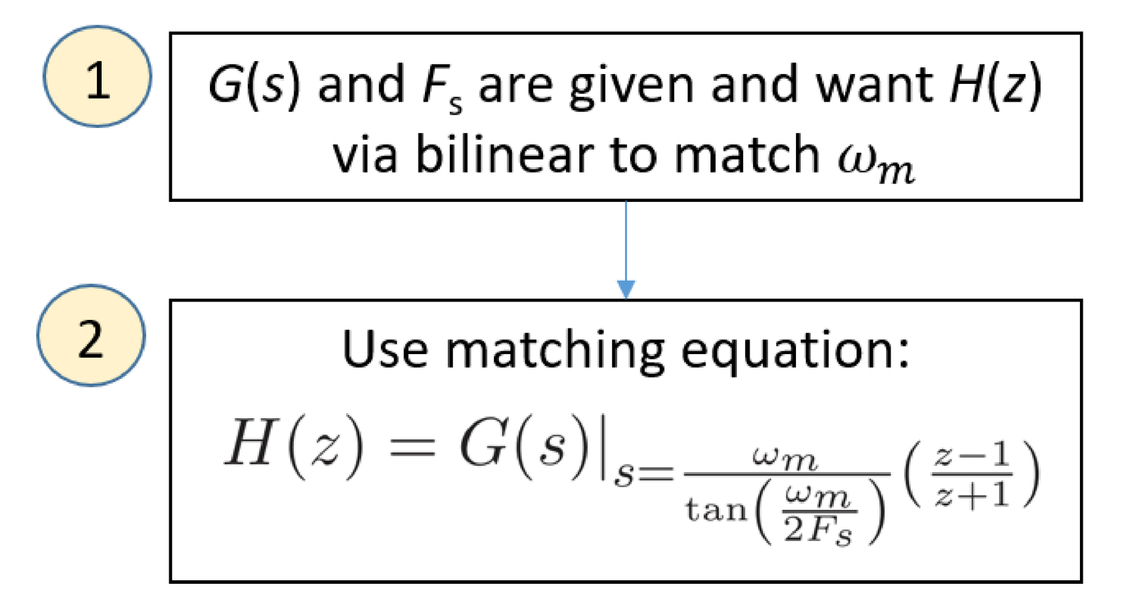
When $G (s)$ and $F_{s}$ are given and there is a single frequency of interest to be “matched” in the continuous and discrete-time domains, it is possible to use $F'_{s}$ to take pre-warping in account and reach a matching between $G (s)$ and $H (z)$ . This “matching” frequency strategy can also be used to design IIR filters when there is a single frequency of interest.

The single “match” frequency $ω_{m}$ is $ω_{m} = ω_{a} = ω_{d}$ rad/s. From Eq. (3.77):

ω_{m} = 2 F_{s} tan (\frac{ω_{m}}{2 F_{s}}),

(3.80)

which can be writte as

F_{s} = \frac{ω_{m}}{2 tan (\frac{ω_{m}}{2 F_{s}})} .

The trick is to consider that $F_{s}$ at the left side is a new value $F'_{s}$ , which can be chosen to impose the matching:

F'_{s} = \frac{ω_{m}}{2 tan (\frac{ω_{m}}{2 F_{s}})},

(3.81)

while $F_{s}$ in the tangent is the provided (original) $F_{s}$ value. Instead of using the angular frequency $ω_{m} = 2 π f_{m}$ , one can use the linear frequency $f_{m} = ω_{m} ∕ (2 π)$ Hz. In summary, the matching can be imposed by³²

F'_{s} = \frac{ω_{m}}{2 tan (\frac{ω_{m}}{2 F_{s}})} = \frac{π f_{m}}{tan (\frac{π f_{m}}{F_{s}})} .

(3.82)

To avoid the discontinuity of $tan (π ∕ 2)$ , one has to choose $\frac{π f_{m}}{F_{s}} < π ∕ 2$ , which corresponds to $F_{s} > 2 f_{m}$ , which is consistent with the sampling theorem. As expected, having a pre-defined $F_{s}$ restricts $f_{m} < F_{s} ∕ 2$ to be less than the Nyquist frequency.

Hence, instead of using Eq. (3.64), it is possible to incorporate pre-warping such that $ω_{m}$ is the match frequency using:

H (z) = G (s) |_{s = \frac{ω_{m}}{tan (\frac{ω_{m}}{2 F_{s}})} (\frac{z - 1}{z + 1})} .

(3.83)

Example 3.33. Simple example of matched $G (s)$ and $H (z)$ at specific frequency $f_{m}$ Hz. Assume $f_{m} = 10$ Hz and $H (z)$ was obtained from $G (s)$ using Eq. (3.83) with sampling frequency $F_{s} = 30$ Hz. Using Eq. (3.82), the value of $H (z)$ at the angle $Ω_{m} = 2 π f_{m} ∕ F_{s} \approx 2.1$ rad matches the value of $G (s) |_{s = j 20 π}$ at $f_{m} = 10$ Hz.

In case $F_{s} = 60$ Hz and $f_{m} = 10$ Hz, then it is at the angle $Ω_{m} = 2 π f_{m} ∕ F_{s} \approx 1.05$ rad that the value of $H (z)$ matches $G (s) |_{s = j 20 π}$ .

In general, for any value of $f_{m} < F_{s} ∕ 2$ , $f_{m}$ is a matching frequency when the bilinear uses Eq. (3.82). $□$

Figure 3.45 is the equivalent of Figure 3.44 for scenarios of bilinear use in which the goal is to match a single frequency and a continuous-time system function $G (s)$ is provided.

Figure 3.45: Steps for matching a single frequency $ω_{m}$ using the bilinear transformation when a continuous-time system function $G (s)$ and $F_{s}$ are provided.

Similar to what was done starting from Eq. (3.80), Eq. (3.75) can also be used to find $F'_{s}$ that maps a specific pair $Ω_{d}$ and $ω_{a}$ as follows:

F'_{s} = \frac{ω_{a}}{2 tan (\frac{Ω_{d}}{2})} .

(3.84)

Adapting Eq. (3.56) to the current notation, the goal of pre-warping a single frequency is to obtain:

H_{z} (e^{j ω_{d} T_{s}}) \approx H_{s} (ω_{a}) .

(3.85)

over the first Nyquist zone (see Section 3.5.7.0).

Some extra examples of the bilinear transform are discussed in the sequel.

Example 3.34. Pre-warping for matching a single frequency applied to the system of Example 3.27. Matching a single frequency using the bilinear function is easily done in Matlab/Octave. For example, the change in frequency of the pole at $ω_{a} = 20$ rad/s in Figure 3.40 can be avoided using [Hz_num, Hz_den] = bilinear(Hs_num, Hs_den, Fs, 20/(2*pi)) instead of [Hz_num, Hz_den] = bilinear(Hs_num, Hs_den, Fs). Figure 3.46 illustrates the result of pre-warping. Note that, because in this case $H_{s} (s)$ is already given, only for a single frequency the bilinear can achieve $ω_{a} = ω_{d}$ , while all others are non-linearly shifted.

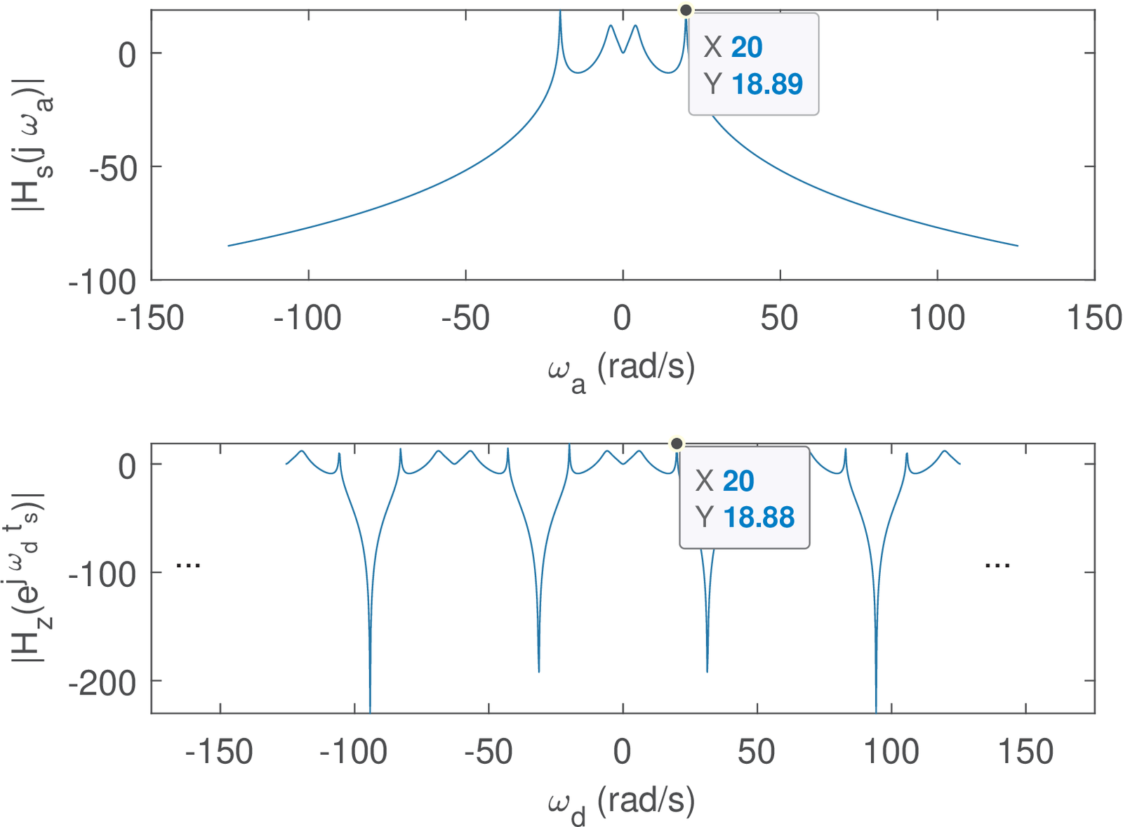
Figure 3.46: Version of Figure 3.40 for which bilinear used pre-warping for obtaining $ω_{a} = ω_{d} = 20$ rad/s.

In this example, there was a single frequency of interest to be matched. If there are several frequencies of interest, they all need to be pre-warped, before the design of $H (s)$ . $□$

Example 3.35. Design an IIR filter by matching a single frequency. The task here is the same as in Example 3.30: design a second-order digital lowpass filter with a 3-dB cutoff frequency of $π ∕ 4$ rad by using the bilinear transformation on the prototype filter $H (s) = 1 ∕ (s^{2} + \sqrt{2} s + 1)$ . There is a single frequency $ω_{m}$ to be matched, which is the cuttof frequency of $H (s)$ . The behavior of $H (s)$ at $ω_{m}$ should match the behavior at $Ω_{m} = π ∕ 4$ of $H (z)$ . Using Eq. (3.84) to match these frequencies leads to $F'_{s} = 1 ∕ (2 tan (π ∕ 8)) \approx 1 ∕ 0.8284 \approx 1.2071$ Hz. Using Eq. (3.64) leads to

\begin{array}{l} H (z) & = \frac{1}{{(\frac{2 \times 1.2071 (z - 1)}{z + 1})}^{2} + \sqrt{2} (\frac{2 \times 1.2071 (z - 1)}{z + 1}) + 1} \\ \approx \frac{0.0976 + 0.1953 z^{- 1} + 0.0976 z^{- 2}}{1 - 0.9428 z^{- 1} + 0.3333 z^{- 2}} . \end{array}

Using Matlab, the following commands implements this shortcut:

1Fs = 1/(2*tan(pi/8)); [Bz,Az]=bilinear(1,[1 sqrt(2) 1],Fs)

which does not explicitly use pre-warping in the bilinear function, but incorporates it on the choice of $F'_{s}$ . $□$

Example 3.36. Pre-warped bilinear applied to a first-order system. Table 3.6 summarized several methods to convert a first-order $H (s)$ into $H (z)$ . Here we extend this table by creating Table 3.8, which incorporates the pre-warped bilinear transformation.

Table 3.8: Pre-warped bilinear as a method to convert

H (s)

into

H (z)


Method	Mapping	$H (z)$ when
		$H (s) = \frac{a}{s + a}$

Bilinear	$s = \frac{2}{T_{s}} (\frac{1 - z^{- 1}}{1 + z^{- 1}})$	$\frac{a}{\frac{2}{T_{s}} (\frac{1 - z^{- 1}}{1 + z^{- 1}}) + a}$

Pre-warped bilinear	$s = \frac{2}{T_{s}} (\frac{1 - z^{- 1}}{1 + z^{- 1}})$ and	$\frac{tan (\frac{a T_{s}}{2})}{(\frac{1 - z^{- 1}}{1 + z^{- 1}}) + tan (\frac{a T_{s}}{2})}$
	$ω_{a} = \frac{2}{T_{s}} tan (\frac{T_{s} ω_{d}}{2})$

The bilinear with pre-warping in Table 3.8 is based on first modifying $H (s)$ using Eq. (3.77). In other words, the pole with cutoff frequency $ω_{c} = a$ in $H (s)$ is pre-warped to obtain $ω_{d} = a$ in the end, after the conversion using bilinear. This is done with $ω_{a} = (2 ∕ T_{s}) tan (T_{s} a ∕ 2)$ and frequency scaling, substituting $s$ by $s ∕ ω_{a}$ . This leads to

H (s) = \frac{\frac{2}{T_{s}} tan (\frac{a T_{s}}{2})}{s + \frac{2}{T_{s}} tan (\frac{a T_{s}}{2})} .

Applying the bilinear mapping to this $H (s)$ leads to the result in Table 3.6.

An alternative shortcut is to use Eq. (3.83) with $ω_{m} = a$ rad/s as the “matching frequency”. This also leads to the result in Table 3.6 $□$

3.13.3 Bilinear for mimicking G(s)

In the following discussion, $G (s)$ is already provided and the bilinear should be used to transform it, or a scaled version of $G (s)$ , into $H (z)$ . An example of application is the task of obtaining a discrete-time version $H (z)$ of a given continuous-time controller $G (s)$ that is applied to a plant. In this case, the sampling frequency can be chosen according, e. g., to the sampling theorem (Eq. (1.30)).

Consider a control system (see [ url3pid]) that uses a PID controller given by

G (s) = 100 + \frac{200}{s} + 10 s .

The dominant pole of the plant $P (s)$ to be controlled³³ is $s = 2$ , which suggests a settling time of approximately 2 seconds. Therefore, the sampling frequency is chosen as $F_{s} = 20$ Hz, which is fast enough when compared to the time constants involved in the dynamics of $G (s)$ . Using bilinear transformation, the digital version of this PID controller is

H (z) = \frac{505 z^{2} - 790 z + 305}{z^{2} - 1},

which should be adjusted for the task of automatic control until the system presents good behavior in closed loop.

In the case of mimicking $G (s)$ , there is not a small set of frequencies of interest as in IIR filter design. The most effective strategy to improve the bilinear transformation and better mimic $G (s)$ is to increase $F_{s}$ to reach a good approximation in Eq. (3.70).

²⁹ When using buttord and butter, Python does not lead to the same results as Matlab/Octave [ url3bor].

³⁰ Matlab tries to match the requirement at the stopband frequency while Python’s SciPy tries to match the requirement at the passband frequency [ url3bor].

³¹ For instance, the bilinear is discussed in [OS09] always in the context of IIR filter design and $F_{s}$ is assumed to be always an arbitrary value.

³² In Matlab (version R2022a), inspecting the source code of the bilinear function with the command type bilinear lists the command sampleFreq = pi*preWarp/tan(pi*preWarp/sampleFreq), which corresponds to Eq. (3.82).

³³ To simplify the discussion, the plant $P (s)$ is not presented here.