Review of Sampling and Signal Reconstruction Using Convolution

3.6 Review of Sampling and Signal Reconstruction Using Convolution

Having established the fundamentals of convolution in this chapter and Fourier transforms in Chapter 2, it is now possible to thoroughly review two stages already introduced in Section 1.7: sampling and reconstruction. The convolution is useful in modeling both stages, which are used in the A/D and D/A processes, respectively.

3.6.1 Sampling as convolution in frequency-domain

As discussed in Chapter 1 (see, e. g. Section 1.5.2), sampling a signal $x (t)$ at each $T_{s}$ seconds (periodic and uniform sampling) can be modeled as the multiplication of $x (t)$ by a periodic function $p (t)$ with fundamental period $T_{s}$ . For example, $p (t)$ can be a train of pulses with duty cycle $T_{1}$ . However, instead of using pulses or other alternatives, it is mathematically convenient¹⁹ to adopt an impulse train

p (t) = \sum_{k = - \infty}^{\infty} δ (t - k T_{s}),

(3.52)

which allows to model the sampled signal as

x_{s} (t) = x (t) p (t) = \sum_{k = - \infty}^{\infty} x (k T_{s}) δ (t - k T_{s}),

(3.53)

as anticipated in Eq. (1.32).

Now we can get extra insight by observing the sampling operation in frequency-domain. In fact, from Eq. (3.53) and the Fourier convolution property discussed in Section 3.3.4, the Fourier transform of $x_{s} (t)$ is

X_{s} (f) = X (f) * P (f),

(3.54)

where $X (f) = F {x (t)}$ and $P (f) = F {p (t)}$ is another impulse train, but in frequency domain. As indicated by Eq. (B.22), the impulses in $P (f)$ are spaced by $F_{s} = 1 ∕ T_{s}$ and have an area equals to $F_{s} = 1 ∕ T_{s}$ .

The convolution of $X (f)$ with the impulses in $P (f)$ creates infinite replicas of $X (f)$ at frequencies values that are multiples of $F_{s}$ as depicted in Figure 3.28. If $F_{s}$ is not sufficiently large, these replicas will overlap and create aliasing. But in case $F_{s} > 2 F_{max}$ , all replicas are “perfect” copies of $X (f)$ scaled by $T_{s}$ .

Figure 3.28: Spectrum $X_{s} (f)$ of a sampled signal $x_{s} (t)$ obtained by the convolution between $X (f)$ and $P (f)$ as indicated in Eq. (3.54).

An alternative view of the sampling process is illustrated in Figure 3.29, which also incorporates the A/DT process.

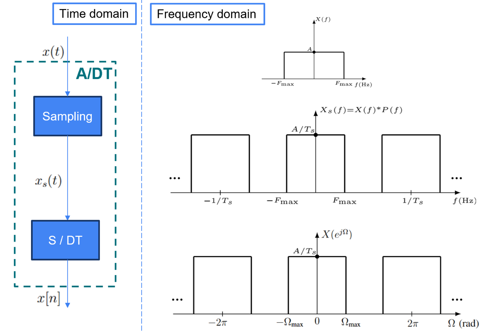
Figure 3.29: Spectra $X (f)$ , $X_{s} (f)$ and $X (e^{j Ω})$ corresponding to the respective time-domain signals $x (t)$ , $x_{s} (t)$ and $x [n]$ observed in a A/DT (analog to discrete-time) conversion.

Figure 3.29 emphasizes that both $x_{s} (t)$ and $x [n]$ have periodic spectra, represented by $X_{s} (f)$ and $X (e^{j Ω})$ , respectively. The fundamental equation Eq. (1.35) provides the mapping between $F_{max}$ in $X_{s} (f)$ and $Ω_{max} = 2 π F_{max} T_{s}$ in $X (e^{j Ω})$ .

3.6.2 Signal reconstruction as convolution in time-domain

The reconstruction process, which converts a sampled signal $x_{s} (t)$ into a continuous-time signal $x (t)$ , was discussed in Section 1.7.7. Now, we are capable of mathematically modeling this process as the convolution of $x_{s} (t)$ with a signal $h (t)$ to obtain $x (t) = x_{s} (t) * h (t)$ . The signal $h (t)$ is the impulse response of the reconstruction (or interpolation) filter, and the reconstruction process can be pictorially depicted as:

x_{s} (t) \to h(t) \to x (t) .

(3.55)

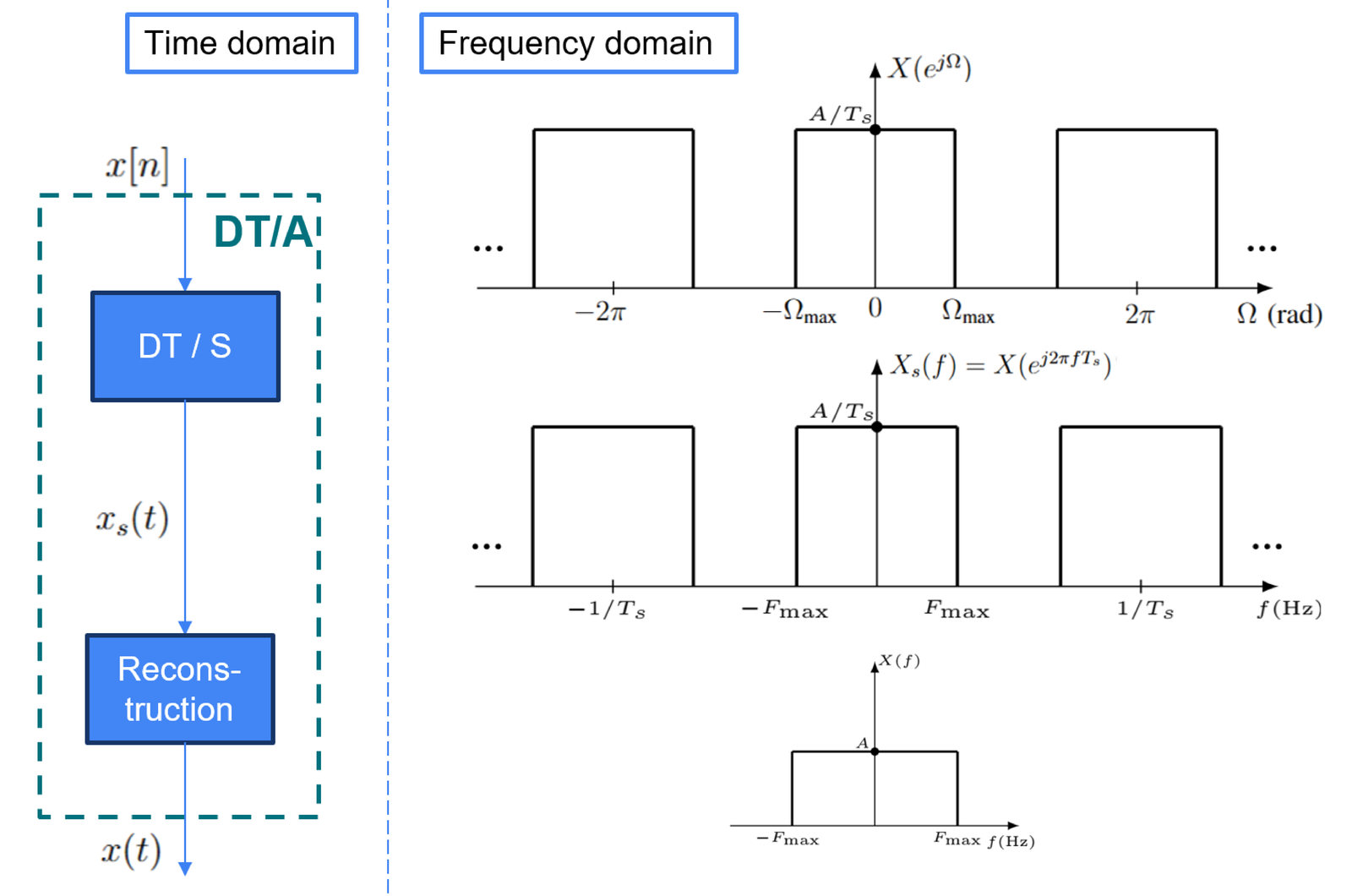
When one starts with the discrete-time signal $x [n]$ , the process has two stages: DT/S conversion, that transforms the discrete-time $x [n]$ into a continuous sampled signal $x_{s} (t)$ and then processed by the reconstruction filter to obtain $x (t)$ , as indicated below:

x [n] \to DT/S \to x_{s} (t) \to h(t) \to x (t) .

(3.56)

Figure 3.30 illustrates the ideal reconstruction process, where the original signal $x (t)$ is recovered by a proper reconstruction stage.

Figure 3.30: Spectra $X (e^{j Ω})$ , $X_{s} (f)$ and $X (f)$ corresponding to the respective time-domain signals $x [n]$ , $x_{s} (t)$ and $x (t)$ observed in a DT/A (discrete-time to analog) conversion and ideal reconstruction.

There are many options for the impulse response $h (t)$ of the reconstruction filter, and the following two important options were discussed in Section 1.7.7:

Zero-order hold reconstruction: where $h (t) = u (t) - u (t - T_{s})$ is a pulse with duration $T_{s}$ and amplitude 1
Sync reconstruction: where $h (t) = sinc (t ∕ T_{s})$ is a sinc with amplitudes equal to zero at $t = \pm T_{s}, \pm 2 T_{s}, \dots$ .

The next section discusses that perfect reconstruction is obtained withe the second option: sync reconstruction.

3.6.3 Perfect reconstruction with the ideal filter (equivalent to sinc interpolation)

After sampling in a way that obeys the sampling theorem (Theorem 1), the original spectrum $X (s)$ can be recovered by a reconstruction filter that operates at $X_{s} (f)$ to keep one replica of the original spectrum and eliminate all others. For perfect reconstruction, this filtering procedure is done with an ideal lowpass filter of bandwidth $BW = F_{s} ∕ 2$ and gain $T_{s}$ , as depicted in Figure 3.31 (which focus on the reconstruction filter of Figure 3.30). The ideal filter in Figure 3.31 will then cancel the undesired replicas of $X_{s} (f)$ and recover $X (f)$ using precisely the scaling factor $T_{s}$ imposed by the spectrum of the pulse train $P (f)$ in Eq. (3.54).

Figure 3.31: Ideal reconstruction filter.

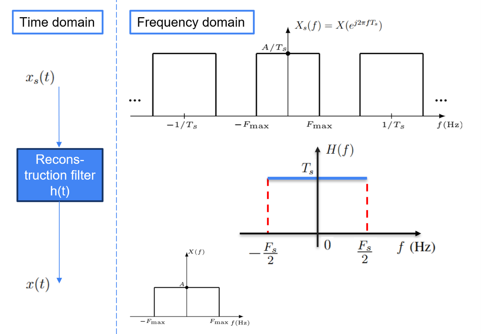
In summary, a lowpass signal $x (t)$ with maximum frequency $F_{max}$ , can be perfectly reconstructed from its sampled version $x_{s} (t)$ if the sampling frequency obeys $F_{s} > 2 F_{max}$ (Theorem 1) and the reconstructed signal $x (t)$ in Figure 3.31 is obtained by passing $x_{s} (t)$ through an ideal lowpass filter with frequency response $H (f)$ having gain $T_{s}$ over the passband.

From Eq. (B.14) and the duality property, the impulse response of this ideal lowpass filter in Figure 3.31 is

h (t) = F^{- 1} {H (f)} = sinc (t ∕ T_{s}) .

This multiplication of $X_{s} (f)$ by $H (f)$ in frequency-domain to obtain $X (f) = X_{s} (f) H (f)$ , corresponds to the convolution of $x_{s} (t)$ with the reconstruction filter’s impulse response $h (t) = sinc (t ∕ T_{s})$ . Hence, this convolution is written as

x (t) = x_{s} (t) * h (t) = \sum_{n = - \infty}^{\infty} x_{s}^{a} (n T_{s}) sinc (\frac{t}{T_{s}} - n),

(3.57)

which corresponds to the convolution of $sinc (t ∕ T_{s})$ with impulses²⁰ of area $x_{s}^{a} (n T_{s})$ . The time shift by $n$ in Eq. (3.57) positions the sincs at $n T_{s}$ , and was discussed in Example 1.5.

Eq. (3.57) represents the reconstruction of a band-limited signal by the sinc interpolation of its samples and is called the Whittaker-Shannon interpolation formula .

Using the notation suggested by Block (3.60), the samples $x (n T_{s})$ were converted to areas $x_{s}^{a} (n T_{s})$ , which are converted to $x [n] = x_{s}^{a} (n T_{s})$ . Hence, Eq. (3.57) can be conveniently rewritten as

x (t) = x_{s} (t) * h (t) = DT/S {x [n]} * h (t) = \sum_{n = - \infty}^{\infty} x [n] sinc (\frac{t}{T_{s}} - n) .

(3.58)

With this background, we can then sketch a proof of the sampling theorem (Theorem 1) in the next section.

3.6.4 A proof sketch of the sampling theorem

The inequality $F_{s} > 2 F_{max}$ of the sampling theorem can be obtained by the following reasoning:

f 1.: Figure 3.29 shows that replicas of the original spectrum $X (f)$ are repeated with period $F_{s}$ .
f 2.: To avoid overlapping replicas, $X (f)$ must be band-limited. Therefore, we assume that $| X (f) | = 0$ when $| f | > F_{max}$ .
f 3.: Observing $X_{s} (f)$ in Figure 3.29, in the range $f \in [0, F_{s}]$ , one must guarantee: a) an interval of $F_{max}$ Hz to the replica centered in $f = 0$ , and b) another interval of $F_{max}$ Hz (from $F_{s} - F_{max}$ to $F_{s}$ ) to accommodate the range originally corresponding to negative frequencies of $X (s)$ due to its replica centered in $f = F_{s}$ .
f 4.: Hence, twice the interval $F_{max}$ must be accomodated within the range $[0, F_{s}]$ , which demands that $F_{s} > 2 F_{max}$ to avoid overlapping replicas.

The condition $F_{s} > 2 F_{max}$ guarantees that there are no overlapping replicas. And Figure 3.31 can be used to illustrate that, according to the sampling theorem, the original signal $x (t)$ can be recovered via an ideal lowpass reconstruction filter. This ideal filter cannot be exactly implemented in practice, but the sampling theorem provides a theoretical result that helps the design of DSP systems that involve sampling.

The previous reasoning also facilitates observing that the sampling theorem uses a strict inequality. Some authors state this theorem as $F_{s} \geq 2 F_{max}$ , but in this case $F_{max}$ would have to be interpreted as the frequency for which $X (f)$ does not have a discrete frequency component $δ (f - F_{max})$ . The confusion often arises when textbooks pictorially represent $X (f)$ with a triangle shape (in contrast, a pulse is used in Figure 3.28) and, in this case, $F_{max}$ is the “maximum” but $X (F_{max}) = 0$ such that $F_{s} \geq 2 F_{max}$ “works”. However, as the exercise of Eq. (1.34) suggests, it is not guaranteed to reconstruct a cosine of frequency $f_{c}$ if one takes its samples at rate $F_{s} = 2 f_{c}$ .

Another source of confusion with respect to $F_{s} \geq 2 F_{max}$ or $F_{s} > 2 F_{max}$ is that when processing a signal sampled at $F_{s}$ with an FFT, the maximum frequency is the so-called Nyquist frequency $F_{s} ∕ 2$ of Table 1.5. Taking that $F_{max} = F_{s} ∕ 2$ , it seems reasonable to adopt $F_{s} \geq 2 F_{max}$ . Note however that the FFT bin corresponding to the Nyquist frequency is representing all signal components within its width $Δ_{f}$ and that, unless $X (f)$ has a discrete frequency component $δ (f - F_{max})$ to create ambiguity as exemplified in Eq. (1.34), there is no major practical issue.

3.6.5 Advanced sampling use cases

Undersampling or passband sampling

Most digital signal processing (DSP) systems are designed to combat aliasing but there are exceptions. In digital communications, it is common to use aliasing to lower the frequency of a signal $x (t)$ in an operation known as undersampling or passband sampling. Among other conditions, $x (t)$ has to be a passband signal with spectrum centered at (a relatively high) frequency $f_{c}$ , but with (a relatively small) bandwidth $BW < f_{c}$ , such that $F_{s} > 2 BW$ . In this case, even if $F_{s} < 2 f_{max}$ , where the maximum frequency is $f_{max} = f_{c} + 0.5 BW$ , $x (t)$ can still be reconstructed from a replica of its spectrum that was shifted in frequency.

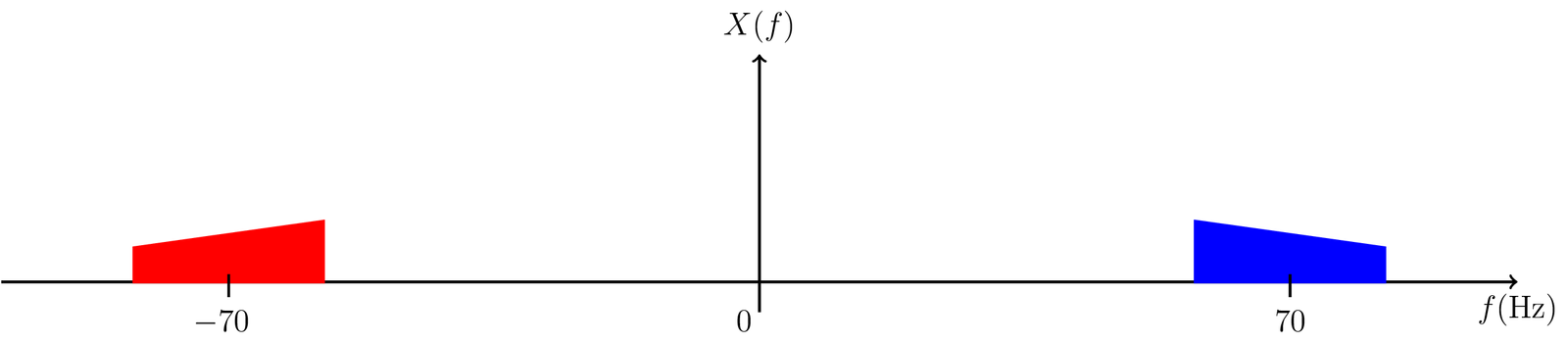
For example, consider a passband signal $x (t)$ with spectrum $X (f)$ with $BW = 25$ Hz and center frequency $f_{c} = 70$ Hz, as depicted in Figure 3.32. This signal has $f_{max} = f_{c} + 0.5 BW = 82.5$ Hz and using the sampling theorem as applied to lowpass signals one would be compeled to use $F_{s} > 2 \times 82.5 = 165$ Hz. However, using $F_{s} = 56$ Hz, for example, one can still recover the signal.

Figure 3.32: Passband signal with $BW = 25$ Hz and center frequency $f_{c} = 70$ Hz.

According to the classic model for the sampling operation, it corresponds to the convolution of $X (f)$ with an impulse train $P (f)$ such that $X_{d} (f) = X (f) * P (f)$ and $P (f)$ has impulses separated by $F_{s} = 56$ . Hence, the sampled signal has spectrum $X_{d} (f)$ as depicted in Figure 3.33.

Assuming $x (t)$ is real and $X (f)$ has Hermitian symmetry, any of the two “replicas” in Figure 3.32 could be used to reconstruct $x (t)$ . Similarly, any of the six (among the infinite) replicas that are shown in Figure 3.33 could be used to reconstruct $x (t)$ .

Figure 3.33: Result of sampling $X (f)$ in Figure 3.32 with $F_{s} = 56$ Hz, which places replicas at $f = \pm 14, \pm 42, \pm, 70, \pm 98, \dots$ , with only the first six shown in this figure.

For example, placing an ideal lowpass filter with cutoff frequency $F_{s} ∕ 2$ would obtain a version of $x (t)$ corresponding to a frequency downconversion of its spectrum $X (f)$ from 70 to 14 Hz.

The theory about undersampling indicates the range of $F_{s}$ that can be used in each situation and can be found in DSP textbooks.²¹

Sampling a complex-valued signal

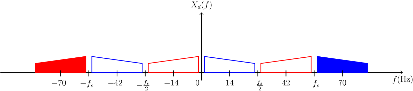
The sampling theorem (Theorem 1) assumed a real-valued signal, which consequently, allowed to assume the spectrum magnitude is even (symmetric). In the more general case of a complex-valued signal, the same principle of having spectrum replicas that cannot overlap is valid, but the “maximum positive frequency” is not enough to determine the minimum $F_{s}$ .

Figure 3.34 suggests an example where a complex-valued signal has spectrum $X (f)$ with support from $- 300$ to 100 Hz. A careless interpretation of the sampling theorem could lead to the erroneous conclusion that $F_{s} > 2 \times 100$ Hz suffices to avoid aliasing. But in this case $F_{s} > 400$ Hz is required to avoid the overlap of spectrum replicas. Figure 3.34 adopts $F_{s} = 450$ Hz.

Figure 3.34: Sampling with $F_{s} = 450$ Hz a complex-valued signal with non-symmetrical spectrum.

Stating the sampling theorem for complex-valued signals requires more elaborated definitions of bandwidth (this is discussed in Section 3.4.6.0). But Figure 3.34 (and Figure 3.28) indicate that an efficient strategy is to follow the basic principle of avoiding aliasing after convolving the original spectrum with the train of impulses spaced by $F_{s}$ .

3.6.6 DSP in practice: analog anti-aliasing and reconstruction filters

The impulse response $h (t)$ of a reconstruction filter can be selected according to the intended application. In analytical derivations, it is often convenient to normalize $h (t)$ to have unit energy, which avoids introducing an additional scaling factor when relating the power of the discrete-time sequence to that of the reconstructed continuous-time signal. For example, the pulse

h (t) = \frac{1}{\sqrt{T_{s}}} [u (t) - u (t - T_{s})]

has unit energy and therefore preserves this normalization. In practical DSP implementations, the signals are not perfectly band-limited as in, e. g., Figure 3.29 in which $| X (f) | = 0$ for $| f | > F_{max}$ . This imposes requirements not only on the reconstruction filter to attenuate the periodic replicas of a sampled signal $X (e^{jω T_{s}})$ , but also demand an efficient anti-aliasing filter to constrain the bandwidth of the input signal $x (t)$ . These requirements are discussed in this section.

Practical DSP systems typically employ two analog filters: an anti-aliasing filter before the ADC and a reconstruction filter after the DAC. The anti-aliasing filter attenuates frequency components above the Nyquist frequency $F_{s} ∕ 2$ , reducing the distortion caused by spectral aliasing during sampling. On the output side, many DACs perform reconstruction internally using a simple ZOH, whose frequency response is often insufficient to suppress the spectral replicas generated by the D/A conversion process. Consequently, an analog reconstruction filter is commonly placed after the DAC to attenuate these undesired images. Rather than focusing on idealized textbook models, this section discusses the practical role of these two filters.

Figure 3.35 presents the extended version of Figure 1.42 that incorporates the filters $A (s)$ and $R (s)$ (these two analog filters are also indicated in Figure 3.22). Figure 3.35 assumes ZOH reconstruction is internally executed by the DAC chip, while the external reconstruction filter has an arbitrary impulse response $r (t)$ .

Figure 3.35: Extended version of Figure 1.42 using a DAC with a ZOH reconstruction filter and incorporating the filters $A (s)$ and $R (s)$ . Quantization is not considered here.

In Figure 3.35, two reconstruction filters are being used: ZOH and $R (s)$ , with impulse response $z (t)$ and $r (t)$ , respectively. Their effect can be eventually combined in a single filter with impulse response $h (t) = z (t) * r (t)$ .

Signal reconstruction with non-ideal filters

The ZOH reconstruction filter with impulse response $z (t)$ in Figure 3.35 represents the filtering process that occurs within a DAC chip. Modern DACs can already incorporate a sophisticated reconstruction filter, but is is assumed hereafter that this is not the case, and $R (s)$ is needed.

The “external” reconstruction filter $R (s)$ in Figure 3.35 complements the ZOH and provides improved rejection of the undesired spectrum replicas of $y_{s} (t)$ that may still be present in $y (t)$ . In summary, the main role of the ZOH is the conversion of the sampled signal $y_{s} (t)$ into an analog signal $y (t)$ , while $R (s)$ aims at achieving the specified level of performance with respect to filtering out the replicas in $y_{s} (t)$ . The following example illustrates how signal reconstruction can be challenging in practice, with non-ideal filters.

Example 3.25. Examples of signal reconstruction. Figure 3.36 is the result of an example²² where a random signal $y [n]$ with $BW = 25$ kHz and $F_{s} = 200$ kHz, is converted to an analog signal $y (t)$ . The reconstruction is performed by a DAC followed by a 5-th order analog filter $H (f)$ , with cutoff frequency $f_{c} = BW$ . This analog filter combines the effects of the ZOH filter and $R (s)$ in Figure 3.35.

The top plot in Figure 3.36 shows the magnitude of the DTFT $Y (e^{2 π T_{s} f})$ of $y_{s} (t) = DT/S {y [n]}$ , superimposed to the frequency response $| H (f) |$ of the reconstruction filter. The multiples of $F_{s}$ are identified in the grid of dashed lines. The bottom plot shows the magnitude of the resulting Fourier transform $Y (f) = F {y (t)}$ .

Figure 3.36: Reconstruction of a digital signal with $BW = 25$ kHz and $F_{s} = 200$ kHz using an analog filter with cutoff frequency $f_{c} = 25$ kHz.

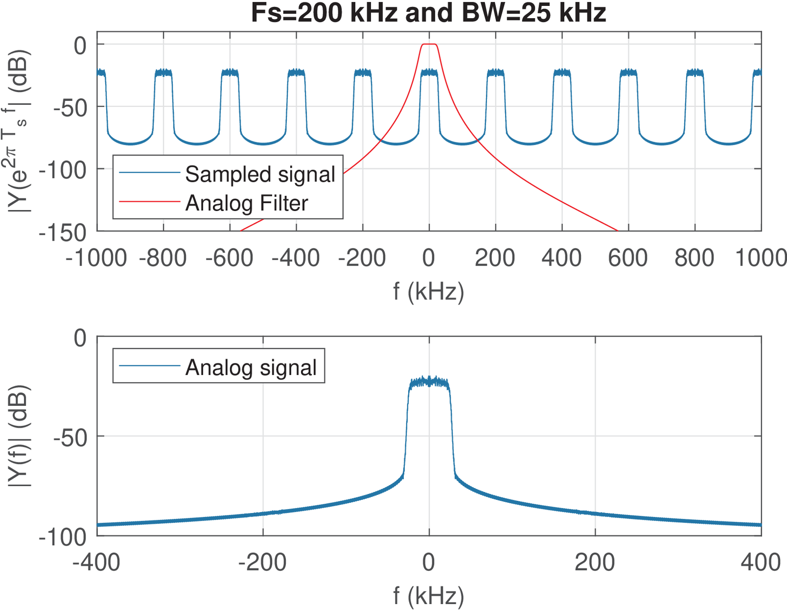
Figure 3.37 was obtained under the same conditions used for Figure 3.36 but the signal bandwidth increased from 25 to 80 kHz. In this case, the filter did not significantly attenuate the two spectrum replicas in $Y (e^{2 π T_{s} f})$ that are neighbors of the one centered at $f = 0$ . Thinking of an asymptotic Bode-diagram, one can expect the fifth-order $| H (f) |$ to drop at 6 dB/octave per pole and, from 80 to 160 kHz, reach $5 \times (- 6) = - 30$ dB. The replica centered at 200 kHz, for example, has its band starting at 120 kHz, and the reconstruction filter has an attenuation of only (approximately) 20 dB at 120 kHz.

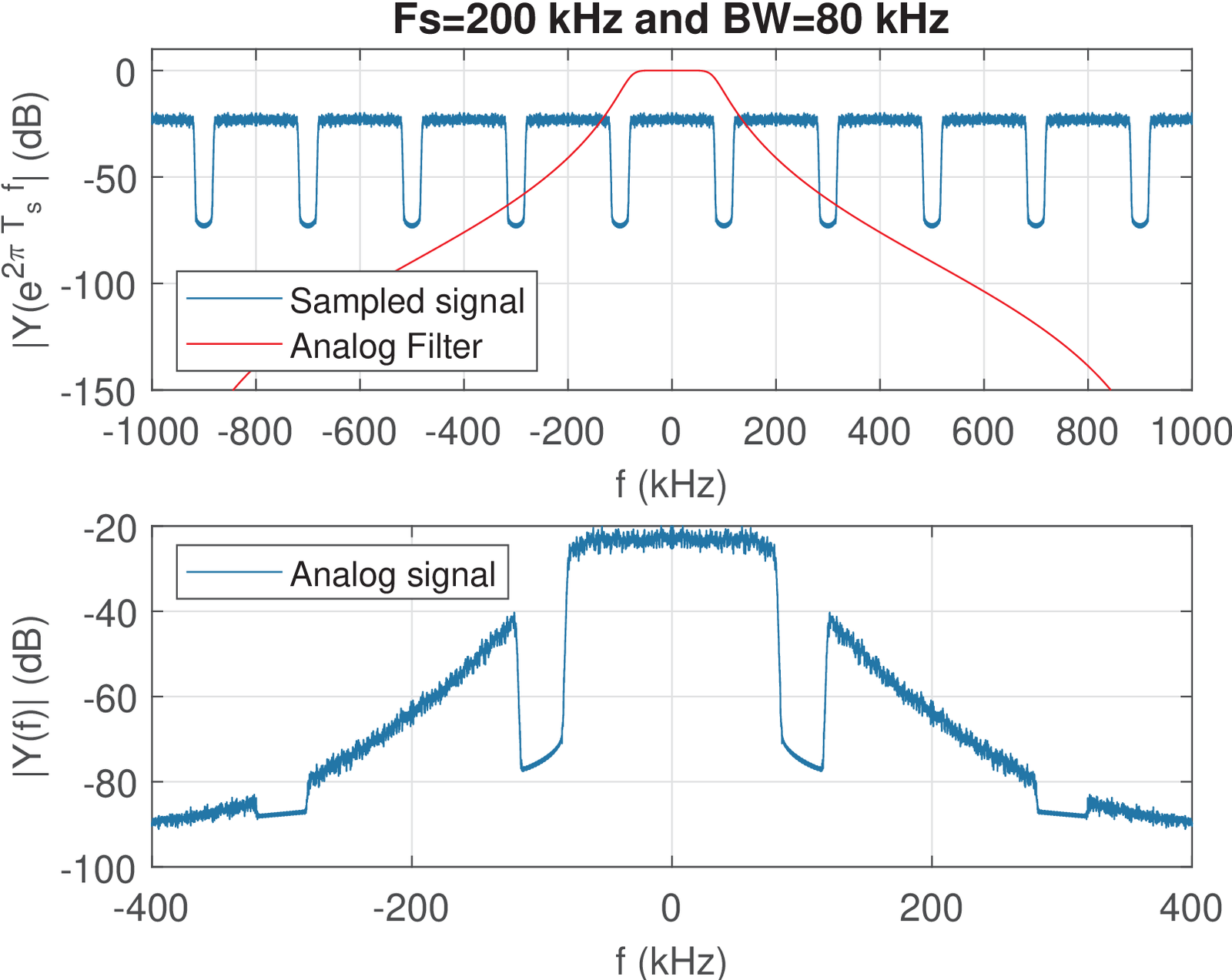
Figure 3.37: Same as Figure 3.36, but for a signal with $BW = f_{c} = 80$ kHz. In this case, the reconstruction generates significant out-of-band power due to the spectrum replicas.

As illustrated by Figure 3.37, in practice, it is typically adopted a value for $F_{s}$ large enough due to the non-ideal reconstruction filter. In the example corresponding to Figure 3.36, in which the reconstruction seems adequate, the Nyquist frequency $F_{s} ∕ 2$ is four times the signal BW. $□$

Oversampled versus critically-sampled signals

As suggested by Figure 3.37, a practical remedy to simplify the design of the reconstruction filter $R (s)$ in Figure 3.35 is the adoption of oversampling.

For a lowpass signal whose highest frequency component is $f_{max}$ , a sampling frequency $F_{s}$ that avoids aliasing obeys $F_{s} > 2 f_{max}$ . The sampling frequency $F_{s} = 2 f_{max}$ is known as the Nyquist rate, and when $F_{s} = 2 f_{max}$ , the signal is said to be critically sampled.

If the spectrum of a critically-sampled signal does not have a discrete component at $f_{max}$ the spectral replicas created by sampling at $F_{s} = 2 f_{max}$ are adjacent but do not overlap, leaving no transition band for a practical reconstruction filter. Consequently, perfect reconstruction in this case requires an ideal lowpass filter with cutoff frequency $F_{s} ∕ 2$ .

In practice, DSP systems typically choose $F_{s} > 2 f_{max}$ rather than sampling at the Nyquist rate. The resulting guard band between adjacent spectral replicas simplifies the design of the reconstruction filter by allowing a finite transition band. For instance, selecting $F_{s} = 4 f_{max}$ doubles the Nyquist rate and provides substantial separation between the baseband spectrum and its replicas.

The following sections discuss issues related to energy and power of signals along the stages of sampling and reconstruction.

3.6.7 Advanced: Energy and power of a sampled signal

The squared of the continuous-time impulse $δ^{2} (t)$ is not defined. This creates a problem when one considers the energy or power of $δ (t)$ . When $δ (t)$ is interpreted as a pulse $p (t)$ with unit area and amplitude $1 ∕ Δ$ , one can argue that when $lim_{Δ \to 0}$ as in Eq. (B.42), the resulting area of the squared pulse $p^{2} (t)$ is $1 ∕ Δ$ , which leads to $δ^{2} (t) = \infty$ . However, this would not be mathematically rigorous given that $δ (t)$ is a distribution. Hence, the following route is taken here: instead of defining new transformations²³ on the distribution $δ (t)$ , the instantaneous power of a sampled signal $x_{s} (t)$ is defined as the instantaneous power of its equivalent discrete-time signal $x [n]$ obtained via a S/DT conversion, normalized by the associated $T_{s}$ , i. e.

P_{s} \overset{def}{=} \frac{P_{d}}{T_{s}} .

(3.59)

For example, the pulse train of Eq. (3.52) has average power $P_{s} = 1 ∕ T_{s}$ because when converted to discrete-time its power is $P_{d} = 1$ .

The same reasoning can be applied to sampled signals for which the independent variable is not $t$ . The Fourier transform $P (f) = {p (t)}$ of Eq. (3.52) has power $1 ∕ T_{s}$ because its discrete-frequency version has power $1 ∕ {T_{s}}^{2}$ and the normalizing factor is $1 ∕ T_{s}$ in this case. Note that, with this definition of instantaneous power of a sampled signal, the power of the impulse trains $p (t)$ and $P (f)$ are the same, as expected from Eq. (B.12).

3.6.8 Advanced: Energy / power conservation after sampling and reconstruction

When the sampling theorem is obeyed, the whole chain is as follows (the signals are depicted with their associated power in parenthesis as in Block (1.75)):

\underset{(P_{c})}{x (t)} \to sampling \to \underset{(P_{s})}{x_{s} (t)} \to S ∕ DT \to \underset{(P_{d})}{x [n]} \to DT ∕ S \to \underset{(P_{s})}{x_{s} (t)} \to h (t) \to \underset{(P_{c})}{x (t)}

(3.60)

where $h (t) = sinc (t ∕ T_{s})$ is the impulse response of the ideal filter depicted in Figure 3.31.

As illustrated in Figure 1.41, DT/S followed by zero-order hold reconstruction is a simplified model for the actual process executed by a DAC chip. A consequence of ZOH is that Eq. (1.77) holds, and the power in continuous $P_{c}$ of $x (t)$ and discrete-time $P_{d}$ of $x [n]$ are the same.

With the help of Eq. (3.58), it is possible to sketch a proof for Eq. (1.77), which is valid when the sampling theorem is obeyed.

Eq. (3.58) states that any band-limited signal $x (t)$ can be represented by its samples $x [n]$ . The interest here is to relate their respective power values $P_{c}$ and $P_{d}$ . Assuming $x (t)$ is an energy signal and from Eq. (A.25), its energy $E_{c}$ can be written as

E_{c} = \int_{- \infty}^{\infty} | x (t) |^{2} d t = \int_{- \infty}^{\infty} {| ∑_{n = - \infty}^{\infty} x [n] sinc (t ∕ T_{s} - n) |}^{2} d t = T_{s} \sum_{n = - \infty}^{\infty} | x [n] |^{2} = T_{s} E_{d},

(3.61)

where $E_{d}$ is the energy of $x [n]$ . A similar reasoning can be applied to power signals. Rewriting Eq. (1.24) with $Δ t = N T_{s}$ leads to

\begin{array}{l} P_{c} & = lim_{N \to \infty} [\frac{1}{(2 N + 1) T_{s}} \int_{- N T_{s}}^{N T_{s}} {| \sum_{n = - N}^{N} x [n] sinc (t ∕ T_{s} - n) |}^{2} d t] \\ = lim_{N \to \infty} [\frac{T_{s}}{(2 N + 1) T_{s}} \sum_{n = - N}^{N} | x [n] |^{2}] \\ = P_{d} . & (3.62) \end{array}

From Eq. (3.62) and Eq. (3.59), Block (3.60) can be simplified as

\underset{(P)}{x (t)} \to sampling \to \underset{(P ∕ T_{s})}{x_{s} (t)} \to S ∕ DT \to \underset{(P)}{x [n]} \to DT ∕ S \to \underset{(P ∕ T_{s})}{x_{s} (t)} \to h (t) \to \underset{(P)}{\hat{x} (t)} = x (t),

(3.63)

where $P = P_{c} = P_{d}$ .

¹⁹ It avoids the “ $sin (x) ∕ x$ ” distortion in frequency domain associated to a pulse train.

²⁰ If needed, recall the notation for sampled signals in Section 1.7.1.

²¹ For example, in [Lyo10].

²² Figure 3.36 and Figure 3.37 were generated with figs_systems_showDACFilterEffect.m, which uses both a low and high sampling frequencies to mimic the reconstruction via an analog filter.

²³ See, e. g., references in Appendix B.6.4.