Introduction to Analog and Digital Filters

3.4 Introduction to Analog and Digital Filters

This section presents some basic concepts of analog and digital filters.

3.4.1 Frequency response: Fourier transform of the impulse response

As indicated in Table 3.1, the frequency response of an LTI system is the Fourier transform of its impulse response. In continuous-time it will be denoted by $H (f)$ ( $f$ in Hz) or $H (ω)$ ( $ω$ in rad/s), while in discrete-time the notation is $H (e^{j Ω})$ ( $Ω$ in rad). The frequency response is particularly useful because complex exponentials are eigenfunctions of LTI systems as explained in the sequel.

Eigenfunctions

Eigenfunctions are closely related to eigenvectors. if $A$ is a matrix (a linear transformation), a non-null vector $x$ is an eigenvector of $A$ if there is a scalar $λ$ such that

A x = λ x .

The scalar $λ$ is an eigenvalue of $A$ corresponding to the eigenvector $x$ . In general, the matrix $A$ generates a completely new vector $y = A x$ , i. e., $y$ and $x$ have different directions and magnitudes. However, if $x$ is an eigenvector of $A$ , then $y = λ x$ , which means that the operation changed only the magnitude of $x$ , leaving its direction unchanged (or possibly reversing it in case $λ < 0$ ).

Similarly, for any LTI system $H$ (continuous-time is assumed here), a complex exponential is an eigenfunction because the output is $y (t) = λ e^{j ω_{0} t}$ when the input is $x (t) = e^{j ω_{0} t}$ . The frequency response is useful because the eigenvalue $λ = H (ω_{0})$ is the value of the frequency response $H (ω)$ at the specific frequency $ω = ω_{0}$ .

It is then possible to analyze an LTI in the frequency domain by following the next steps:

f 1.: Using the Fourier transform $X (ω) = F {x (t)}$ to decompose a non-periodic input $x (t)$ as an integral of complex exponentials.
f 2.: Obtain the frequency response $H (ω) = F {h (t)}$ of the system with impulse response $h (t)$ . The frequency response $H (ω)$ provides the eigenvalue $H (ω_{0})$ for any input $e^{j ω_{0} t}$ of frequency $ω_{0}$ .
f 3.: Conceptually, multiply each complex exponential $e^{j ω_{0} t}$ at the system input by its eigenvalue $H (ω_{0})$ and add the partial results to obtain the system output $y (t)$ . In practice, this step is performed by $Y (ω) = H (ω) X (ω)$ and then using the inverse transform to obtain $y (t) = F^{- 1} {Y (ω)}$ .

The previous steps are slightly different in case the input signal is periodic. In this case, the Fourier series is used to represent the input signal as a summation (instead of an integral) of complex exponentials.

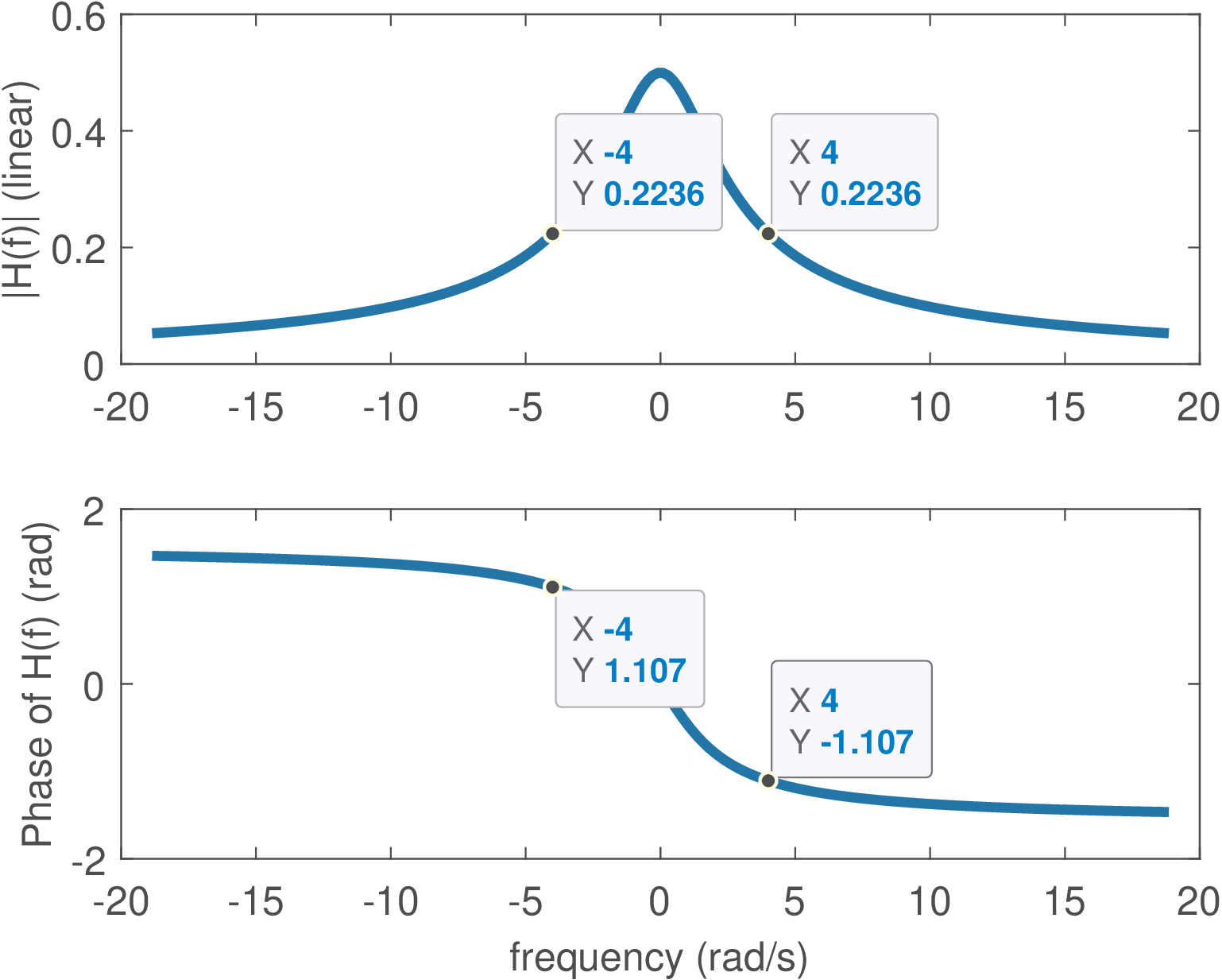
Figure 3.5: Frequency response of $H (ω) = \frac{1}{jω + 2}$ represented in polar form: magnitude (top) and phase (bottom). The data tips indicate the values for $ω = \pm 4$ rad/s.

Example 3.7. LTI filtering of continuous-time complex exponential. For example, consider that $x (t) = 6 e^{j 4 t} + 6 e^{- j 4 t} = 12 cos (4 t)$ is the input of an LTI with $h (t) = e^{- 2 t} u (t)$ . The eigenvalues corresponding to each the complex exponential eigenfunctions with frequencies $ω = \pm 4$ rad/s can be obtained from the frequency response $H (ω) = F {h (t)} = \frac{1}{jω + 2}$ . The Matlab/Octave commands Omega=4; H=1/(j*Omega+2) calculate $H (ω) |_{ω = 4} = 0.1 - 0.2 j$ for the positive frequency. Because $h (t)$ is real-valued, the frequency response presents Hermitian symmetry and $H (ω) |_{ω = - 4} = H^{*} (ω) |_{ω = 4}$ , i. e., $H (ω) |_{ω = - 4} = 0.1 + 0.2 j$ . The commands abs(H), angle(H) can be used to convert the complex numbers from the Cartesian to the polar representation: $H (ω) |_{ω = 4} \approx 0.2236 e^{- j 1.107}$ and $H (ω) |_{ω = - 4} \approx 0.2236 e^{j 1.107}$ . Therefore, the output is $y (t) = (0.2236 e^{- j 1.107}) 6 e^{j 4 t} + (0.2236 e^{j 1.107}) 6 e^{- j 4 t} = 1.32 e^{j (4 t - 1.11)} + 1.32 e^{j (- 4 t + 1.11)} = 2.64 cos (4 t - 1.11)$ .

The effect of the LTI system was to impose to the input $x (t)$ a gain of $| H (4) | = 0.2236$ and a phase of $∠H (4) = - 1.107$ rad that shows up at the output $y (t)$ . Figure 3.5 depicts the frequency response for a range $ω = 2 π [- 3, 3]$ rad/s. Because of the Hermitian symmetry (when $h (t)$ is real), it is common to plot only the positive frequencies. For example, investigate the command freqs(1,[1 2]), which shows the frequency response of $H (ω) = \frac{1}{jω + 2}$ in a different format. $□$

Result 3.1. LTI systems cannot create new frequencies. The previous discussion implies that an LTI never creates new frequencies, because it can simply change the magnitude and phase of frequencies that were presented at its input. This fact can be represented as

e^{j ω_{0} t} \to H \to H (ω_{0}) e^{j ω_{0} t} .

Note that a linear time-varying (LTV) system can generate new frequency components, just as a nonlinear time-invariant (NLTI) system can. Only when a system is both linear and time-invariant (LTI) does the restriction apply that no new frequencies can be created. $□$

The previous discussion was restricted to exponentials of the form $e^{j ω_{0} t}$ , but a general complex exponential $e^{st}$ (with $σ \neq 0$ ) is also an eigenfunction of any LTI and the eigenvalue is given by the Laplace transform $H (s)$ , as represented by

e^{s_{0} t} \to H \to H (s_{0}) e^{s_{0} t} .

The frequency response $H (e^{j Ω})$ of discrete-time LTI systems is also very useful. When the time axis $t$ is discretized by sampling, i. e., $t = n T_{s}$ , the complex exponential $e^{st}$ becomes $e^{sn T_{s}}$ , which is more conveniently represented by $z^{n}$ , where

z = e^{s T_{s}}

with $z, s \in ℂ$ .

The discrete-time complex exponential $z^{n}$ is an eigenfunction of discrete-time LTI systems. To prove that, consider $x [n] = {(z_{0})}^{n}, z_{0} \in ℂ$ , then

\begin{array}{l} y [n] & = \sum_{k = - \infty}^{\infty} {(z_{0})}^{k} h [n - k] = ∑_{k = - \infty}^{\infty} h [k] {(z_{0})}^{n - k} = {(z_{0})}^{n} ∑_{k = - \infty}^{\infty} h [k] {(z_{0})}^{- k} \\ = {(z_{0})}^{n} H (z) |_{z = z_{0}} . \end{array}

The eigenvalue $H (z) |_{z = z_{0}}$ can be obtained from the transfer function

H (z) = \sum_{n = - \infty}^{\infty} h [n] z^{- n},

which is the Z-transform of the system’s impulse response. As a special case, when $| z | = 1$ , the eigenfunction $e^{j Ω n}$ has its amplitude and phase eventually modified by a LTI as depicted by:

e^{j Ω_{0} n} \to H \to H (e^{j Ω_{0}}) e^{j Ω_{0} n} .

Example 3.8. LTI filtering of discrete-time complex exponentials. This example describes how an LTI system filters a complex exponential. Consider that $x [n] = 4 e^{j 0.5 πn} + 4 e^{- j 0.5 πn} = 8 cos (0.5 πn)$ is the input of an LTI with $h [n] = 0 . 7^{n} u [n]$ . The eigenvalues can be obtained from $H (e^{j Ω}) = F {h [n]} = \frac{1}{1 - 0.7 e^{- j Ω}}$ when $Ω = 0.5 π$ rad. The Matlab/Octave commands omega=pi/2; H=1/(1-0.7*exp(-j*omega)) calculate $H (e^{j Ω}) |_{Ω = 0.5 π} = 0.6711 - 0.4698 j$ . Because $h [n]$ is real-valued, the frequency response presents Hermitian symmetry. The commands abs(H), angle(H) can transform from Cartesian to polar: $H (e^{j Ω}) |_{Ω = 0.5 π} \approx 0.8192 e^{- j 0.6107}$ . Therefore, the output is $y [n] = (0.8192 e^{- j 0.6107}) 4 e^{j 0.5 πn} + (0.8192 e^{j 0.6107}) 4 e^{- j 0.5 πn} = 3.2769 e^{j (0.5 πn - 0.6107)} + 3.2769 e^{j (- 0.5 πn + 0.6107)} = 6.5539 cos (0.5 πn - 0.6107)$ . The effect of the LTI system was to impose a gain of $0.8192$ and a phase of $- 0.6107$ rad.

Figure 3.6: Frequency response of $H (e^{j Ω}) = \frac{1}{1 - 0.7 e^{- j Ω}}$ represented in polar form: magnitude (top) and phase (bottom). The data tips indicate the values for $Ω = π ∕ 2$ rad.

Figure 3.7: Version of Figure 3.6 obtained with the command freqz(1,[1 -0.7]).

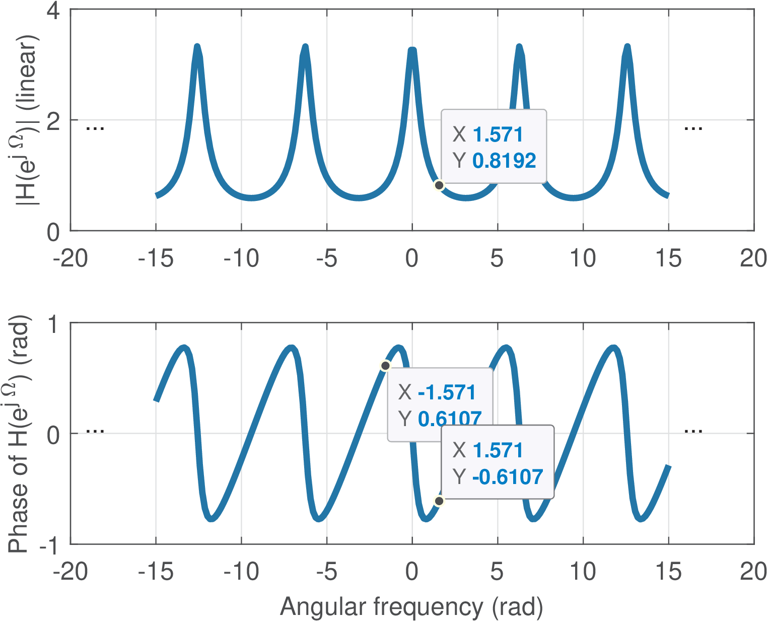
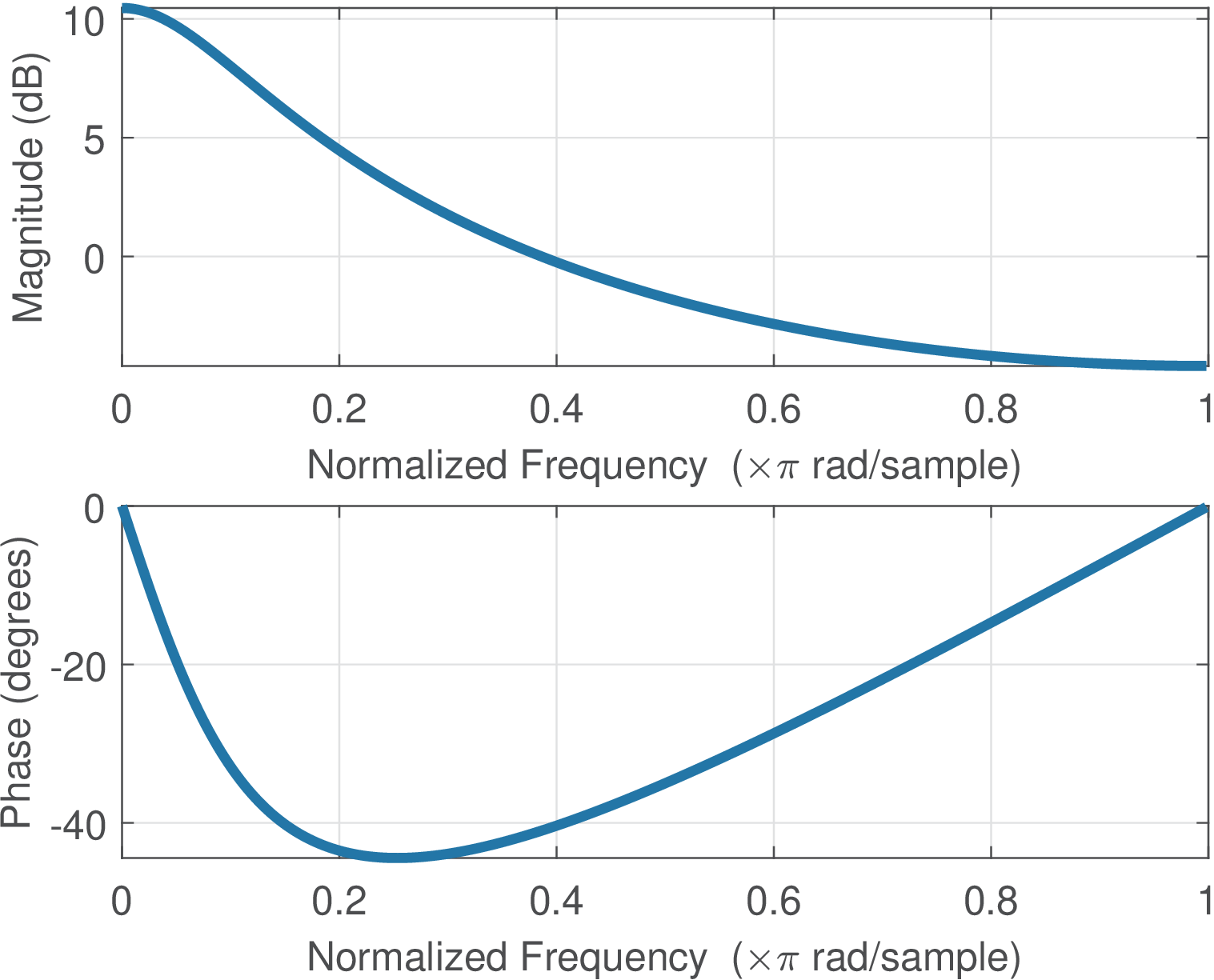
Figure 3.6 depicts the frequency response for a range $Ω = [- 15, 15]$ rad. As expected, $H (e^{j Ω})$ is periodic because $H (e^{j Ω}) = H (e^{j (Ω + 2 π)})$ . Given this periodicity and the Hermitian symmetry (when $h [n]$ is real), it is common to plot only the positive frequencies in the range $Ω = [0, π]$ . For example, Figure 3.7 shows the plots obtained with the command freqz(1,[1 -0.7]), which shows the frequency response of $H (e^{j Ω})$ with the magnitude in dB, the phase in degrees (instead of rad) and the abscissa in a “normalized frequency” $Ω ∕ π$ that maps $[0, π]$ into $[0, 1]$ . $□$

3.4.2 A quick discussion about analog filters

This section presents a brief introduction to a special class of systems called LTI filters, which typically have the characteristic of being frequency-selective. LTI systems will be further discussed in Section 3.3 but the goal here is to provide concrete examples on frequency-selective filters, due to their importance in DSP. Other filters will be discussed, but this section starts with the two most common filters: lowpass and highpass.

The lowpass filter is characterized by attenuating (or rejecting) the frequency components that are above a given frequency called bandpass frequency $f_{p}$ , while providing a gain $κ > 0$ to the frequency components from 0 to $f_{p}$ . The name lowpass is used because the filter allows the low-frequency components of $x (t)$ to “pass” and compose the output. Similarly, the highpass tries to reject the components of $x (t)$ that are located from 0 to its $f_{p}$ in the frequency spectrum, while keeping those higher than $f_{p}$ .

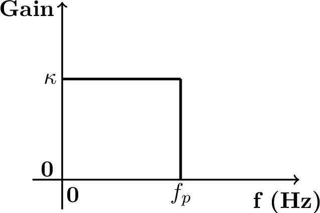
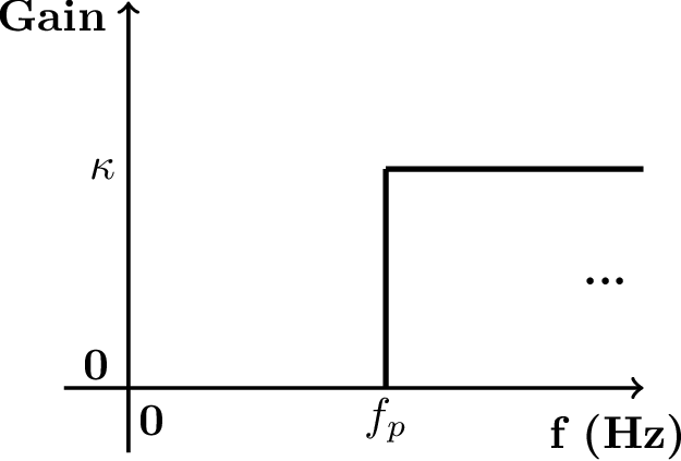
Figure 3.7a and Figure 3.7b depict the ideal specification of low and highpass filters, respectively. These figures only illustrate the magnitude (gain $κ$ ) and, at this moment, the phase $Θ$ is assumed to be zero.

Example 3.9. Lowpass and highpass filtering examples. For example, assume a signal $x (t) = 3 cos (2 π 100 t) + 8 cos (2 π 200 t)$ ( $t$ in seconds) is the input to the lowpass filter of Figure 3.7a with $κ = 1$ , $Θ = 0$ and $f_{p} = 150$ Hz. The output would be $y (t) = 3 cos (2 π 100 t)$ because the component of frequency 200 Hz would be filtered out. If the same $x (t)$ is the input to the highpass filter of Figure 3.7b with $κ = 4$ , $Θ = 0$ and $f_{p} = 190$ Hz, the output would be $y (t) = 32 cos (2 π 200 t)$ . In this case, besides eliminating the lowpass component, the filter imposed a gain of 4 to the amplitude of the 200 Hz component. $□$

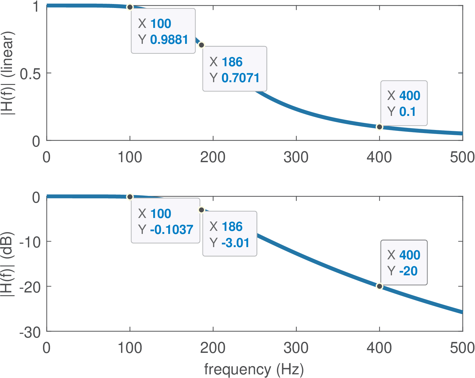
Figure 3.9 shows the magnitude of the frequency response of a (second order analog) filter. This figure should be contrasted to the ideal case of Figure 3.8. In practice the filter gain cannot instantaneously change from 1 to 0 as idealized in Figure 3.8. Instead, this variation (the attenuation rolloff) depends on the filter order and creates a transition region that is defined as the range of frequencies between $f_{p}$ and the stopband frequency $f_{r}$ .

Figure 3.9: Magnitude of the frequency response of a practical analog filter in linear scale ( $| H (f) |$ , top) and in dB ( $20 \log_{10} | H (f) |$ ), which should be compared to the ideal case of Figure 3.8. Three frequencies are of interest: passband ( $f_{p} = 100$ Hz), cutoff ( $f_{c} = 158.5$ Hz) and stopband ( $f_{r} = 500$ Hz) frequencies.

3.4.3 Cutoff and natural frequencies

Besides $f_{p}$ and $f_{r}$ , another frequency of interest is the so-called cutoff frequency $f_{c}$ . Assuming the filter gain at the passband is $κ$ , the cutoff is the frequency for which the linear gain is $κ ∕ \sqrt{2} \approx 0.707 κ$ . The cutoff indicates the frequency in which the filter attenuates a signal component to half of its power at the passband center. For example, assume an input signal $x (t)$ has a component $A cos (2 π f_{c} t)$ with power $A^{2} ∕ 2$ , which is passed through a highpass filter with unitary gain at passband and cutoff frequency $f_{c}$ . This component will show up at the filter output as $\frac{A}{\sqrt{2}} cos (2 π f_{c} t)$ , which has power $\frac{A^{2}}{4}$ , corresponding to half of the original power. In dB scale, the cutoff frequency corresponds to a gain of $20 \log_{10} (1 ∕ \sqrt{2}) \approx - 3.01$ dB, as illustrated in Figure 3.9 for a lowpass filter with gain $κ = 1$ at DC.

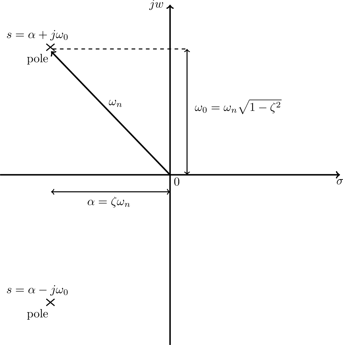
The cutoff frequency should not be confused with the natural frequency, which is detailed in Figure 3.10. Table 3.2 is a useful reference for the special frequencies used in signal processing.

Table 3.2: Nomenclature of special frequencies used in filtering.


Symbol	Description	Reference

$ω_{c}$ or $f_{c}$	Cutoff frequency: where gain falls by $1 ∕ \sqrt{2} \approx 0.707$ ( $- 3$ dB)	Figure 3.9

$ω_{n}$	Natural frequency, for example, of a resonator	Figure 3.10

$ω_{0}$	Center frequency of a pole	Figure 3.10

$f_{p}$	Passband frequency	Figure 3.9

$f_{r}$	Stopband (or rejection) frequency	Figure 3.9

$F_{s}$	Sampling frequency (typically in Hz or samples per sec.)	Eq. (1.26)

$F_{s} ∕ 2$	Nyquist (or folding) frequency	Eq. (2.36)

3.4.4 First and second-order analog systems

Because they are basic building blocks for higher-order systems, first and second-order continuous-time (also called analog) systems are discussed in this section.

First-order systems

If the coefficients are real, a first-order system $H (s) = 1 ∕ (s + a), a \in ℝ$ , (as the one whose frequency response is depicted in Figure 3.5) is restricted to have a lowpass frequency response. This $H (s)$ has a pole at $s = - a$ and a zero at $s = \infty$ . Using $H (s) = a ∕ (s + a)$ leads to a unitary gain at DC. Placing a zero at $s = 0$ leads to $H (s) = s ∕ (s + a)$ , which has a highpass response.

A system $H (s) = 1 ∕ (s + a)$ with ROC given by $σ > - a$ has an inverse Laplace transform $h (t) = e^{- at} u (t)$ , which can be written as $h (t) = e^{- t ∕ τ} u (t)$ where $τ$ is the well-known time constant [ url3mit] of the system’s impulse response. After an interval of one time constant, the impulse response has decayed to 36.8% of its initial value.

If the ROC of $H (s) = a ∕ (s + a)$ includes $s = jω$ , the frequency response in this case is $H (ω) = a ∕ (jω + a)$ . As illustrated by Eq. (3.24), the magnitude $| H (ω) | = a ∕ \sqrt{a^{2} + ω^{2}}$ at $ω = a$ is then $| H (a) | = 1 ∕ \sqrt{2}$ , which is the cutoff frequency $ω_{c} = a$ because it corresponds to a decrease of 3 dB in power.

Second-order systems

The system function $H (s)$ of a second-order system (SOS), also called a two-pole resonator, has a denominator that can be written as $s^{2} + 2 αs + ω_{n}^{2}$ . When there are two zeros at $\infty$ and the gain at DC is unitary ( $H (s) |_{s = 0} = 1$ ), the SOS is:

H (s) = \frac{ω_{n}^{2}}{s^{2} + 2 αs + ω_{n}^{2}},

(3.17)

where $ω_{n}$ is the natural frequency and $α$ the decay rate parameter, which is useful for defining the damping ratio $ζ = α ∕ ω_{n}$ . Hence, Eq. (3.17) can be rewritten as:

H (s) = \frac{ω_{n}^{2}}{s^{2} + 2 ζ ω_{n} s + ω_{n}^{2}} .

(3.18)

Example 3.10. Second-order Butterworth filter. For a generic second-order system, the natural frequency $ω_{n}$ , the pole frequency $ω_{0}$ , and the cutoff frequency $ω_{c}$ are generally different. However, for a Butterworth lowpass filter, the damping ratio is $ζ = 1 ∕ \sqrt{2}$ , and the transfer function can be written as

H (s) = \frac{ω_{0}^{2}}{s^{2} + \sqrt{2} ω_{0} s + ω_{0}^{2}} .

In this special case, the magnitude response satisfies $| H (ω_{0}) | = 1 ∕ \sqrt{2}$ , corresponding to a $- 3$ dB attenuation relative to the passband gain. Therefore, the cutoff frequency coincides with the pole frequency: $ω_{c} = ω_{0}$ .

For example, a second-order Butterworth filter with $ω_{0} = 2 π \times 1000$ rad/s has a cutoff frequency $f_{c} = ω_{0} ∕ (2 π) = 1000$ Hz. $□$

The values of $α$ , $ζ$ and $ω_{n}$ can be related to several characteristics of a SOS. For example, $α$ represents the rate of exponential decay of oscillations when the system input is a unit step $u (t)$ . And depending on $ζ$ , three categories of second-order systems are defined:

$ζ = 1$ : critically damped SOS, with a double real pole at $- ω_{n}$ ;
$ζ > 1$ : overdamped SOS, with real poles at $- ζ ω_{n} \pm ω_{0}$ ;
$0 \leq ζ < 1$ : underdamped SOS, with complex conjugate poles.

Note that these three categories depend only on the denominator of $H (s)$ .

The numerator of $H (s)$ represents another degree of freedom. Changing this numerator, leads to distinct SOS. An alternative to Eq. (3.17) (or, equivalently, Eq. (3.18)) is

H (s) = \frac{s}{s^{2} + 2 ζ ω_{n} s + ω_{n}^{2}},

(3.19)

which has a zero at the origin ( $H (s) |_{s = 0} = 0$ ). Yet, other two options of SOS can be defined as

H (s) = \frac{s^{2}}{s^{2} + 2 ζ ω_{n} s + ω_{n}^{2}}

(3.20)

and

H (s) = \frac{2 ζ ω_{n} s + ω_{n}^{2}}{s^{2} + 2 ζ ω_{n} s + ω_{n}^{2}} .

(3.21)

Table 3.3 summarizes these options for the numerator of a SOS.

Table 3.3: Some distinct options for the numerator of a SOS.


Characteristic	Numerator	Reference

Two-zeros at $\infty$ and unitary DC gain	$ω_{n}^{2}$	Eq. (3.18)

One zero at DC	$s$	Eq. (3.19)

Two zeros at DC	$s^{2}$	Eq. (3.20)

One finite zero at $- ω_{n} ∕ (2 ζ)$	$2 ζ ω_{n} s + ω_{n}^{2}$	Eq. (3.21)

Using the quadratic formula to find the roots of a SOS, the poles are $s_{0} = - α \pm \sqrt{α^{2} - ω_{n}^{2}}$ , which can be rewritten as $s_{0} = - α \pm j \sqrt{ω_{n}^{2} - α^{2}}$ . Figure 3.10 summarizes these relations. Note that $ω_{n} = | s_{0} |$ and, unless $α = 0$ (poles on the $jω$ axis), the natural frequency $ω_{n}$ is different from the center frequency of the pole $ω_{0} = I mag {p} = \sqrt{ω_{n}^{2} - α^{2}} = ω_{n} \sqrt{1 - ζ^{2}}$ .

Figure 3.10: Relations between natural frequency $ω_{n}$ , pole center frequency $ω_{0}$ , decay rate $α$ and damping ratio $ζ$ for a pair of complex conjugate poles.

Note that for a first-order system $H (s) = a ∕ (s + a)$ with real-valued coefficient $a$ , the pole is real, its center frequency is $ω_{0} = 0$ , and the natural and cutoff frequencies $ω_{n} = ω_{c} = a$ coincide. For a second-order system, the expression for the cutoff frequency $ω_{c}$ is more elaborated. Considering Eq. (3.17), the cutoff is

ω_{c} = ω_{n} \sqrt{1 - 2 ζ^{2} + \sqrt{4 ζ^{4} - 4 ζ^{2} + 2}},

(3.22)

which can be found by using $| H (s) |_{s = j ω_{c}} = 1 ∕ \sqrt{2}$ . In this case, $ω_{c} = ω_{n}$ when $ζ = 1 ∕ \sqrt{2}$ .

Example 3.11. On the damping ratio of a SOS. Figure 3.11 illustrates the influence of the damping ratio using the values $ζ = 0.5, 0.707, 1$ and 2.

Figure 3.11: Magnitude of the frequency response for the SOS expressed by Eq. (3.18) and Eq. (3.21).

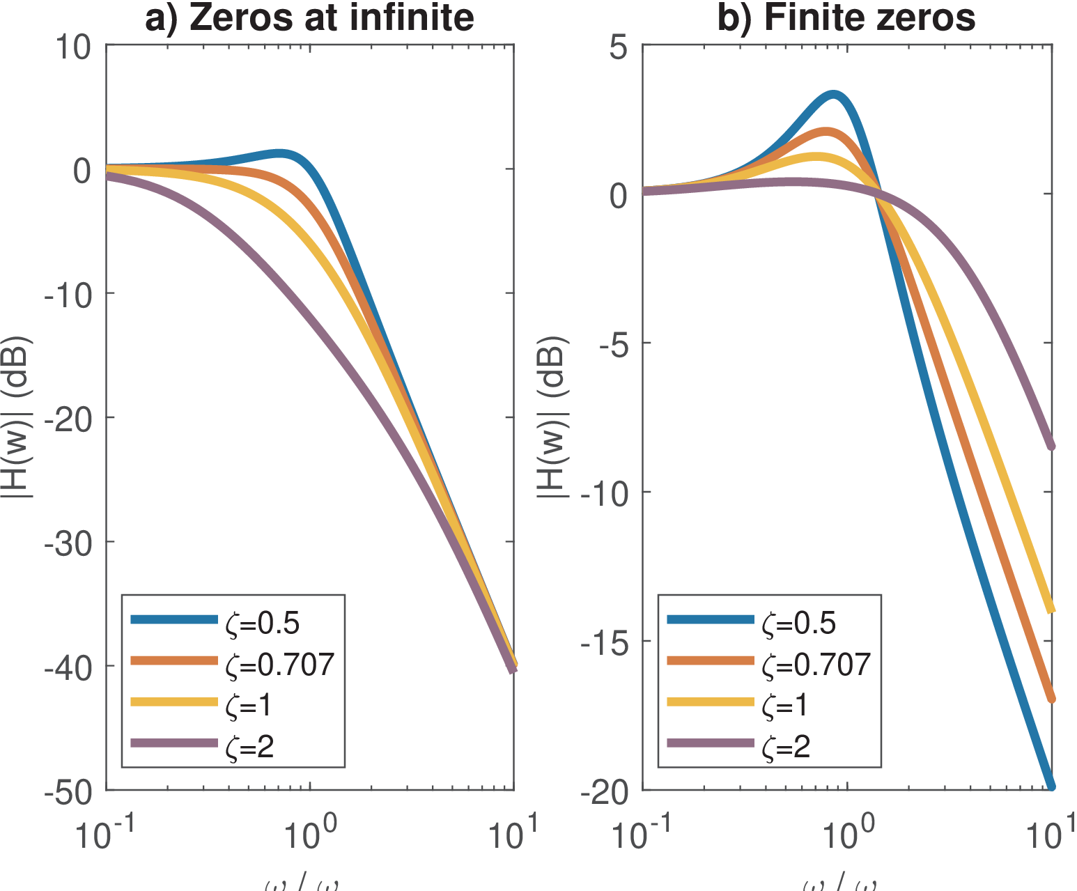
Figure 3.11 also compares Eq. (3.18) and Eq. (3.21), which are two of the options contrasted in Table 3.3. $□$

Figure 3.12 illustrates some key time-domain performance parameters for an underdamped system obtained when the input $x (t) = u (t)$ is a step function. The rise time $t_{r}$ is the interval for the step response to rise from 10 to 90% of its final value. The settling time $t_{s}$ is the interval to have the output within a given range, which is 5% in Figure 3.12. The overshoot is the peak amplitude and occurs at the peak time $t_{p}$ .

Figure 3.12: Time-domain performance parameters for an underdamped system based on its step response.

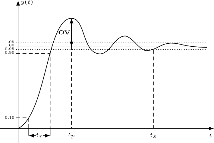
Table 3.4 summarizes some parameters for the system $H (s)$ described by Eq. (3.18), which can be found³ from the inverse Laplace transform of $Y (s) = H (s) ∕ s$ given that $X (s) = 1 ∕ s$ is the transform of $u (t)$ . The tolerance $𝜖$ is used to obtain $t_{s}$ and a typical value is $𝜖 = 0.05$ .

Table 3.4: Parameters of a second-order system as described by Eq. (3.18).


Performance parameter	Expression	For $ζ = \sqrt{2} ∕ 2 \approx 0.707$

Peak time	$t_{p} = π ∕ ω_{0} = π ∕ (ω_{n} \sqrt{1 - ζ^{2}})$	$t_{p} = 4.4 ∕ ω_{n}$

Rise time	$t_{r} \approx (2.23 ζ^{2} - 0.078 ζ + 1.12) ∕ ω_{0}$	$t_{r} = 3 ∕ ω_{n}$

Settling time	$t_{s} = - ln (𝜖 \sqrt{1 - ζ^{2}}) ∕ (ζ ω_{n})$	$t_{s} = 4.7 ∕ ω_{n}$

Overshoot	$ov = e^{- (ζπ) ∕ \sqrt{1 - ζ^{2}}}$	ov=4.32%

3-dB bandwidth $ω_{c}$ (rad/s)	$ω_{c} = ω_{n} \sqrt{1 - 2 ζ^{2} + \sqrt{2 - 4 ζ^{2} + 4 ζ^{4}}}$	$ω_{c} = ω_{n}$

Table 3.4 indicates that, for an underdamped system, the rise time when $ζ = \sqrt{2} ∕ 2$ is $t_{r} = 3 ∕ ω_{n}$ . As expected, all three time parameters are inversely proportional to the natural frequency $ω_{n}$ .

Listing 3.8 indicates the commands to calculate the parameters, emphasizing the factors that depend on $ζ$ (zeta) only.

Listing 3.8: MatlabOctaveCodeSnippets/snip_systems_sos_parameters.m. [ Python version]

1zeta=0.5 %damping ratio, e.g. sqrt(2)/2 = 0.707; 
2wn=2 %natural frequency in rad/s 
3epsilon=0.05 %tolerance for the settling time (5% in this case) 
4tp_factor=pi/sqrt(1-zeta^2) %depends on zeta only 
5tp=tp_factor/wn %peak time 
6tr_factor=(2.23*zeta^2 - 0.078*zeta + 1.12)/sqrt(1-zeta^2) %zeta only 
7tr=tr_factor/wn %rise time 
8ts_factor= -log(epsilon * sqrt(1-zeta^2))/(zeta) %zeta only 
9ts=ts_factor/wn %settling time 
10ov=exp(-(zeta*pi)/sqrt(1-zeta^2)) %overshoot (depends on zeta only) 
11bw_factor=sqrt(1-2*zeta^2 + sqrt(2 - 4*zeta^2 + 4*zeta^4)) %zeta only 
12wc=wn*bw_factor %cutoff frequency=3-dB bandwidth (in radians/second) 
13%% Check whether the cuttoff frequency wc corresponds to a -3 dB gain 
14s = 1j*wc %define s = j wc 
15Hs = (wn^2) / (s^2 + 2*zeta*wn*s + (wn^2)) % system function 
16gain_at_wc = 20*log10(abs(Hs))  %answer is -3.0103 dB

Matlab has the stepinfo function, which can be used to obtain most of the parameters in Table 3.4 as follows:

1zeta=0.5 %damping ratio, e.g. sqrt(2)/2 = 0.707; 
2wn=2 %natural frequency in rad/s 
3sys = tf([wn^2],[1 2*zeta*wn wn^2]); %define the transfer function 
4S=stepinfo(sys,'RiseTimeLimits',[0.1,0.9], ... 
5    'SettlingTimeThreshold',0.05) %get parameters with stepinfo 
6step(sys) %plot step response to check results if want

The system bandwidth will be discussed in the next section. Table 3.4 informs that, when $ζ = \sqrt{2} ∕ 2$ , the 3-dB bandwidth $ω_{c}$ in radians per second of the SOS given by Eq. (3.18) is simply its natural frequency $ω_{n}$ . In fact, as $ζ$ varies from 0.5 to 0.8, which are the values typically used, its $ω_{c}$ varies from $1.27 ω_{n}$ to $0.87 ω_{n}$ . This justifies using $ω_{n}$ as a rough approximation of bandwidth for Eq. (3.18).

Example 3.12. Basic filtering using an electronic circuit simulator. The Falstad’s circuit simulator [ url3fac] can help learning analog filters. In the menu bar, choose Circuits and look for the options in Passive Filters and Active Filters. For instance, Figure 3.12a illustrates a simple low-pass filter with cutoff frequency $f_{c} = 85.11$ Hz. The signal source (at the left) is a sine sweep that generates⁴ sinudoids from 20 Hz to 1kHz during a sweep time of 100 ms. In the figure, the current input signal corresponds to a sinusoid with frequency of 885.1 Hz. As shown by the two scopes in the bottom of Figure 3.12a, this sinusoid at 885.1 Hz is clearly attenuated by this filter given that the amplitude of the output signal is significantly smaller than the input signal amplitude.

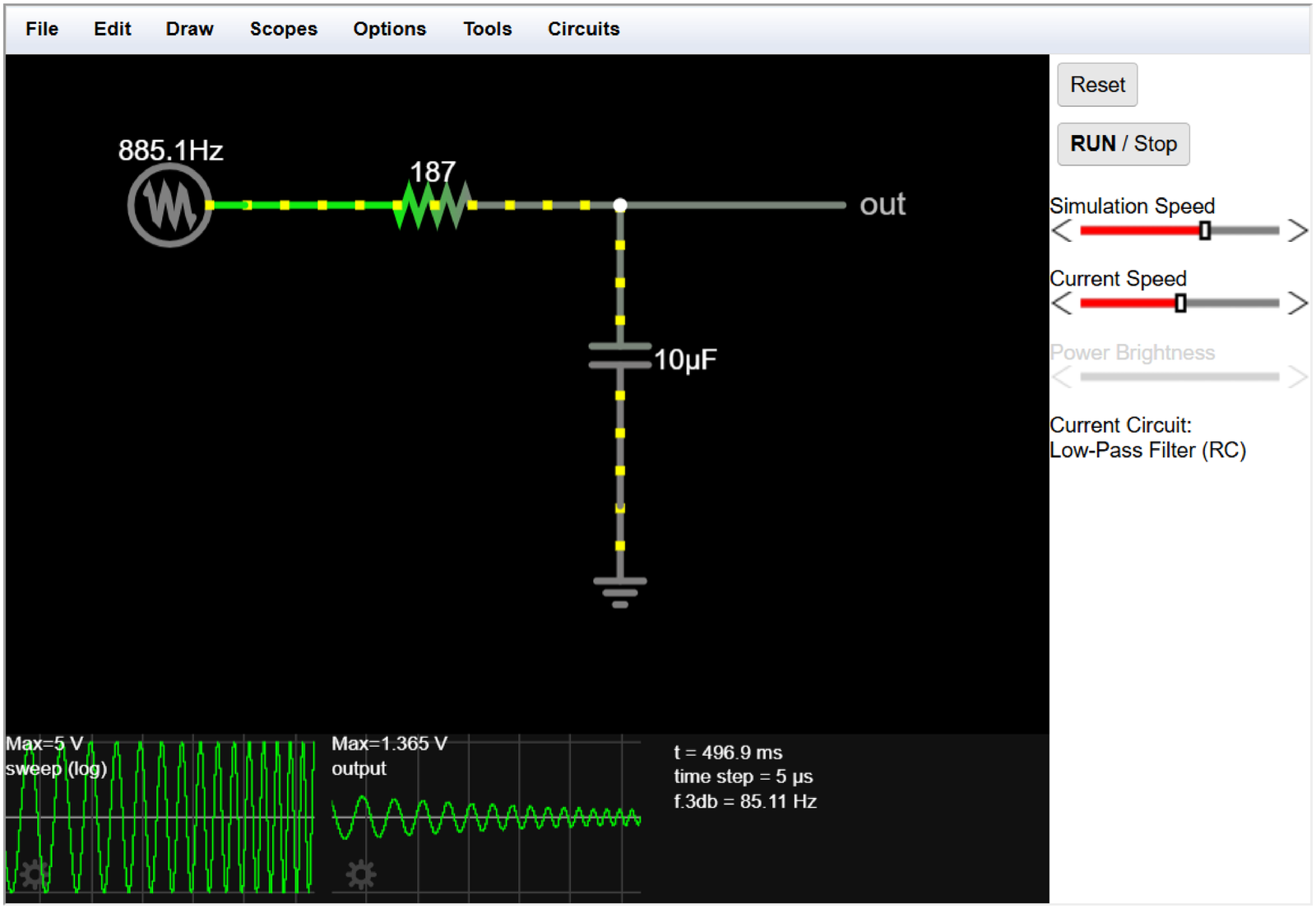
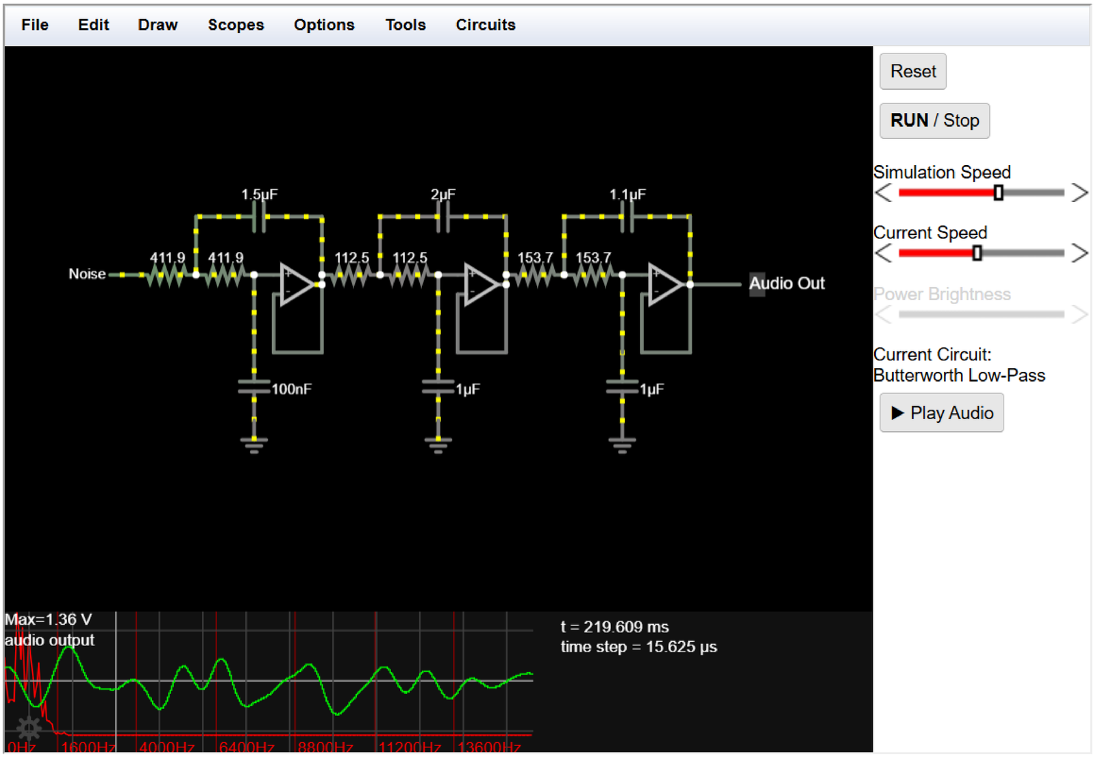
Figure 3.12b shows an example of an active low-pass filter with order equals to six.⁵ The input source generates noise and the scope at the bottom shows the time-domain signal output (in green) and its spectrum (in red). The reader is invited to browse this site and learn with the simulator. $□$

3.4.5 Bandwidth and quality factor

Bandwidth and quality factor of poles

The overall behavior of a filter is dictated by the combined effect of its poles and zeros. The position of a pole in the $s$ or $Z$ plane determines how it influences the overall system function ( $H (s)$ or $H (z)$ , respectively).

It can be shown that asymptotically each pole contributes with a roll-off of 20 dB per decade (equivalent to 6 dB per octave) and a zero with an increase of 20 dB per decade. This asymptotic behavior is used to obtain graphs known as Bode diagrams. This clearly indicates that the sharpness of a frequency response (shorter transition regions) can be improved by increasing the order of the corresponding system function $H (s)$ (or $H (z)$ ), i. e., adding poles and/or zeros. However, increasing the order of an analog filter requires more components (capacitors, opamps, etc.) and for a digital filter it requires more multiplications and additions. Hence, it is important to make the best use of poles (and zeros) and, motivated by that, to have figures of merit for them.

Besides its frequency, the bandwidth and quality factor of a single pole or zero are important to assess its influence. Poles will be emphasized in this section, but similar definitions are applied to zeros. This section discusses characteristics of a single pole while Section 3.4.6 extends the definitions to filters.

Bandwidth of a pole

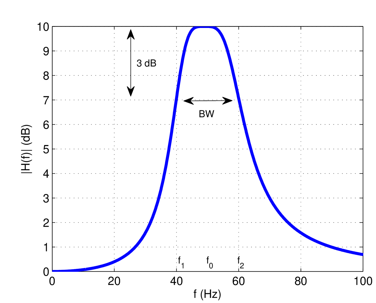
The bandwidth of a pole is illustrated in Figure 3.14 and defined here as $BW = f_{2} - f_{1}$ , where the cutoff frequencies $f_{1}$ and $f_{2}$ are those in which the gain $| H (f_{0}) |$ at the center frequency $f_{0}$ (that may be different than the natural frequency $f_{n}$ ) has decreased to $| H (f_{0}) | ∕ \sqrt{2}$ . The factor $1 ∕ \sqrt{2}$ corresponds to $20 \log_{10} (1 ∕ \sqrt{2}) - 3.0103$ dB, or approximately $- 3$ dB. Therefore, this definition is called the 3-dB bandwidth or half-power BW.

Figure 3.14: Bandwidth $BW = f_{2} - f_{1}$ defined by the cutoff frequencies where the gain falls $- 3$ dB below the reference value at $f_{0}$ .

Pole bandwidth in continuous-time

Assuming a first-order system $H (s) = - α ∕ (s - p)$ , where $p = α + j ω_{0}$ is the pole, the bandwidth of $p$ in Hz is given by

BW = \frac{| α |}{π} .

(3.23)

This result can be obtained by noting that for any frequency $ω$

| H (ω) | = \frac{| α |}{\sqrt{{(ω - ω_{0})}^{2} + α^{2}}} .

Hence, the squared gain at the specific pole frequency $ω = ω_{0}$ is

| H (ω_{0}) |^{2} = \frac{α^{2}}{{(ω_{0} - ω_{0})}^{2} + α^{2}} = 1

and the squared gains at cutoff frequencies $ω = ω_{0} \pm α$ fall to $1 ∕ 2$ as required by the definition of cutoff frequency:

| H (ω_{0} \pm α) |^{2} = \frac{α^{2}}{{(ω_{0} \pm α - ω_{0})}^{2} + α^{2}} = \frac{1}{2} .

(3.24)

Hence, a range from $ω_{0} - α$ to $ω_{0} + α$ is determined by the two cutoff frequencies of a pole at $ω_{0}$ such that its bandwidth $BW$ is $2 | α |$ rad/s. Dividing by $2 π$ leads to $BW = 2 | α | ∕ (2 π)$ in Hz, as indicated in Eq. (3.23). A similar relation holds in discrete-time, as follows.

Pole bandwidth in discrete-time

Using the previous results and assuming the transformation $z = e^{s T_{s}}$ of Eq. (2.66), the pole $p = α + j ω_{0}$ in the plane $s$ is mapped into the pole $z = r e^{j Ω_{0}}$ in the plane $Z$ via

r e^{j Ω_{0}} = e^{p T_{s}} = e^{(α + j ω_{0}) T_{s}} = e^{α T_{s}} e^{j ω_{0} T_{s}} .

Hence, $r = e^{α T_{s}}$ and $Ω_{0} = ω_{0} T_{s}$ . Assuming $α < 0$ for a causal and stable $H (s)$ , Eq. (3.23) indicates that $α = - BW π$ , such that $r = e^{α T_{s}} = e^{- BW π T_{s}}$ and

BW = - \frac{ln (r)}{π T_{s}}

(3.25)

in Hz for a pole $r e^{j Ω_{0}}$ in the $Z$ plane with $r < 1$ .

One can rewrite Eq. (3.25) as $ln (r) = - BW π T_{s}$ and use the Taylor series expansion of $ln (\cdot)$ around a value $x = a$

ln (x) = ln (a) + \frac{1}{a} (x - a) - \frac{1}{2 a^{2}} {(x - a)}^{2} + \frac{1}{3 a^{3}} {(x - a)}^{3} - …,

with $a = 1$ , to keep only the first two terms and achieve

ln (r) \approx ln (1) + \frac{1}{1} (r - 1) = r - 1 .

Hence, the approximation $r - 1 \approx - BW π T_{s}$ allows to write

BW \approx \frac{(1 - r) F_{s}}{π},

(3.26)

which can be used when $r$ is close to 1.

Quality factor of poles

Besides the number of poles and zeros, another factor that influences the sharpness of a frequency response is the quality factor (or $Q$ -factor) of each pole, which is defined as

Q \overset{def}{=} \frac{f_{n}}{BW},

(3.27)

where $f_{n} = ω_{n} ∕ (2 π)$ is the natural frequency in Hz and $BW = f_{2} - f_{1}$ is the 3-dB bandwidth (also in Hz), as indicated in Figure 3.14.

For a second-order resonator, such as Eq. (3.17), the quality factor can be shown [ url3dsp] to be

Q = \frac{ω_{n}}{2 α} .

(3.28)

Appplication 3.1 presents a discussion on the influence of the Q-factor in frequency responses.

3.4.6 Bandwidth and quality factor of filters

The previous definitions of bandwidth and Q-factor of poles can be extended to systems, especially frequency-selective filters such as bandpass and lowpass.

Bandwidth definitions for signals and systems

For a generic system there are definitions for the bandwidth ( $BW$ ) other than the 3-dB bandwidth of Figure 3.14. In all cases, if the frequency response has Hermitian symmetry, only the positive frequencies are taken in account.

A generalization of BW is to adopt the $X$ -dB bandwidth where $X$ is the attenuation of interest, such as 1 dB.

Alternatively, the absolute bandwidth can be applied when the signal is bandlimited. It is simply defined as the frequency range in which the spectrum is non-zero. For example, $H (f) = rect (f)$ has $BW = 0.5$ . Note that in this case the 3-dB BW definition would not be appropriate.

Another alternative definition of $BW$ is the so-called null-to-null or zero-crossing BW. In the case of a lowpass spectrum, the BW is determined by the first null of $| H (ω) |$ (or $| H (Ω) |$ in discrete-time). For example, a frequency response given by the $H (f) = sinc (fT)$ of Eq. (B.14) has $BW = 1 ∕ T$ according to this definition. For a passband spectrum, the two neighbor nulls of the center frequency determine BW. For example, the BW of $H (f) = sinc (fT - 5 T)$ is $BW = 2 ∕ T$ .

When a signal is complex-valued, its spectrum $X (f)$ does not have to exhibit Hermitian symmetry. In this case, the sampling theorem and other results depend on the double-sided or bilateral bandwidth, which takes in account the support of $X (f)$ from negative to positive frequencies.

For example, first consider the “conventional” case of $X (f)$ corresponding to a real-valued ideal lowpass filter with unitary gain from $- 200$ to 200 Hz: its BW is 200 Hz, and its double-sided bandwidth is 400 Hz. Contrast now with a complex-valued signal with $X (f)$ being a square pulse from $- 300$ to 100 Hz as depicted in Figure 3.34. In the latter case, the double-sided bandwidth continues to be 400 Hz but the conventional BW fails to indicate, for example, the minimum $F_{s}$ according to the sampling theorem. In this case, the sampling theorem could be stated with respect to the double-sided bandwidth.

Another approach when dealing with complex-valued signals is to assume that $X (f)$ is zero for negative frequencies (such signals are called “analytic”). In this case, the bandwidth BW takes in account only positive frequencies, as usual, but it may be misleading the fact that the sampling theorem in this case of an analytic signal can be stated as

F_{s} > BW .

(3.29)

For example, if $X (f)$ is non-zero from DC to 300 Hz, sampling the corresponding complex-valued (analytic) time-domain signal $x (t)$ at $F_{s} = 350$ Hz suffices to avoid aliasing. In this case, the first spectrum replica at positive frequencies has support from 0 to 300 Hz, the second one from 350 to 650 Hz, and so on, indicating that there is no aliasing.

A bandwidth definition very useful when dealing with filtered white noise is the equivalent noise bandwidth (ENBW). The ENBW of a filter $H (f)$ is the bandwidth of a fictitious ideal (e. g., lowpass or bandpass) filter $H_{e} (f)$ with rectangular spectrum that obeys

\int_{- \infty}^{\infty} | H (f) |^{2} d f = \int_{- \infty}^{\infty} | H_{e} (f) |^{2} d f

(3.30)

and has the maximum value $H_{max}$ of $| H_{e} (f) |$ is equal to the maximum of $| H (f) |$ . The name ENBW is because both filters lead to the same output power when the input is white noise (discussed in details later, in Section 4.7.2 ) such that the equivalent filter can substitute the original (and more complicated one) while leading, for instance, to the same SNR in a simulation or theoretical development.

An example is provided in Figure 3.15, which was obtained with Matlab’s function⁶ enbw as informed in Listing 3.9. In this case, the ENBW was $102.4 ∕ 50 \approx 2$ times larger than the cutoff frequency.

Listing 3.9: Code/MatlabBookFigures/figs_digicomm_enbw

1Fs = 1000; %sampling frequency in Hz 
2fc = 50; %filter cutoff frequency in Hz 
3[B,A]=butter(4,fc/(Fs/2)); %4-th order Butterworth filter 
4N=100; %number of samples in impulse response hn 
5hn = impz(B,A,100); %impulse response 
6Hf = fftshift(fft(hn)); %sampled DTFT 
7equivalentBW = enbw(hn,Fs); %estimate equivalent noise bandwidth 
8%code to plot the figure continues from here...

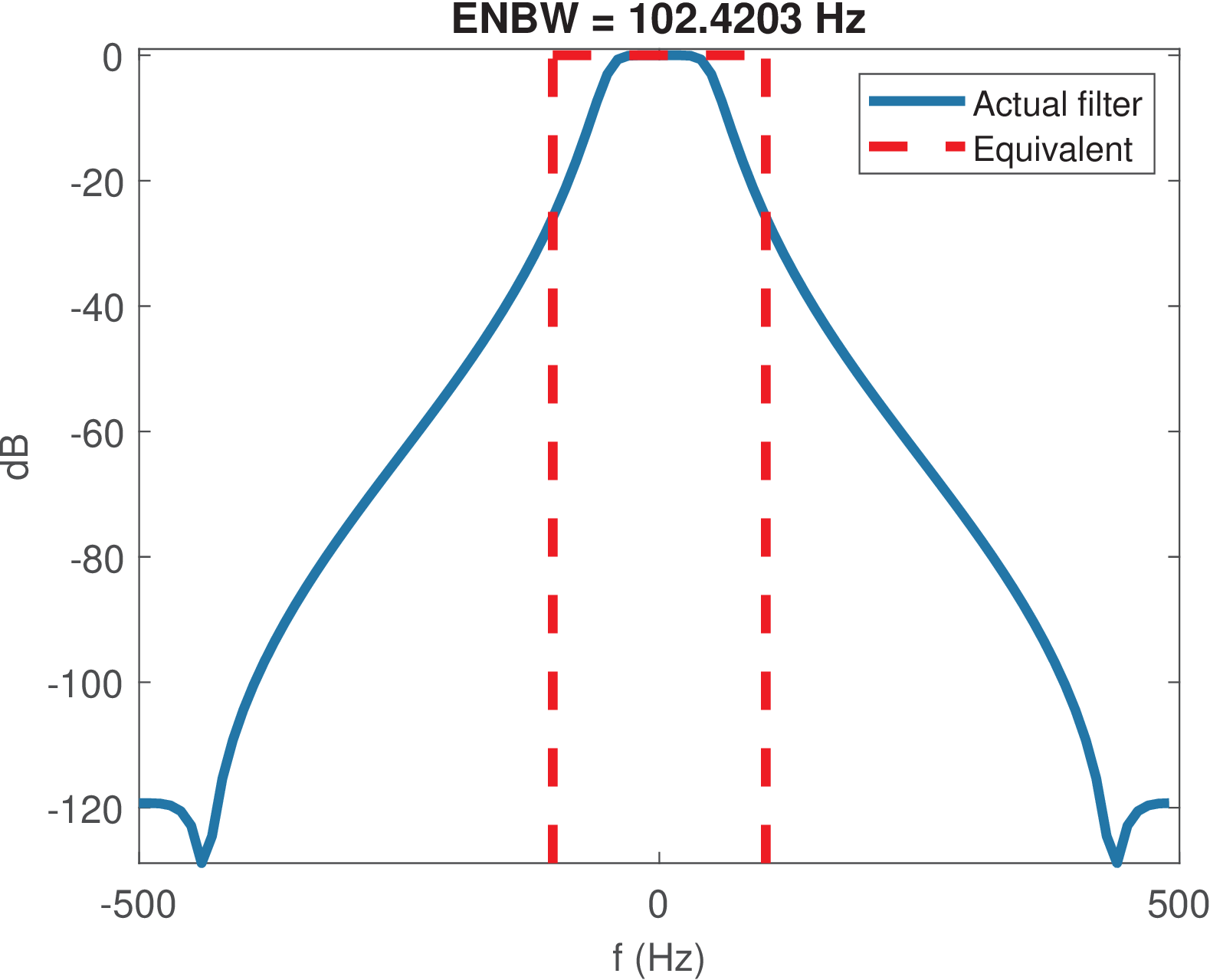
Figure 3.15: DTFT magnitude in dB of a 4-th order Butterworth filter with cutoff frequency of 50 Hz and the equivalent ideal filter with absolute bandwidth of 102.4 Hz.

Observing Figure 3.15, due to the rectangular shape of $| H_{e} (f) |$ ,

\int_{- \infty}^{\infty} | H_{e} (f) |^{2} d f = 2 ENBW \times H_{max}^{2} .

Hence, using Eq. (3.30) this can be written as:

ENBW = \frac{\int_{- \infty}^{\infty} | H (f) |^{2} d f}{2 H_{max}^{2}},

(3.31)

which for real signals simplify to

ENBW = \frac{\int_{0}^{\infty} | H (f) |^{2} d f}{H_{max}^{2}} .

(3.32)

Quality factor for filters

The Q-factor of a pole, as defined in Eq. (3.27), can be easily adapted to a system with a frequency response that allows obtaining its 3-dB bandwidth $BW$ (see Figure 3.14) such as a bandpass filter.⁷ In this case, the pole natural frequency $f_{n}$ in Eq. (3.27) is substituted by the filter’s center frequency $f_{c}$ such that

Q \overset{def}{=} \frac{f_{c}}{BW} .

(3.33)

The inverse of $Q$ , i. e., $BW ∕ f_{c}$ is called fractional bandwidth and often specified in percentage.

3.4.7 Importance of linear phase (or constant group delay)

In some applications such as analog signal transmission and audio amplification, the system should ideally have an output $y (t)$ identical to its input $x (t)$ . Given that obtaining $y (t) = x (t)$ is often unfeasible due to propagation delays inherent of communication channels and electronic systems, a more realistic target is to obtain $y (t) = x (t - t_{0})$ , a delayed version of the input. From the time-shift Fourier property (see Appendix B.1), the delay by $t_{0}$ corresponds to a linear phase $e^{- j 2 πf t_{0}}$ in frequency domain. Hence, having a linear phase is an important property of a system to achieve distortionless transmission, i. e., letting a signal pass without distortion.

A linear phase filter with frequency response $H (ω)$ has a phase $Θ = ∠H (ω)$ that corresponds to a line segment in the passband (the phase behavior in the stopband is considered irrelevant). In practice, the line has a negative slope because a positive slope would correspond to a non-causal behavior (the output would be an anticipated version $x (t + t_{0})$ of the input signal). Hence, it is convenient to define the group delay as:

τ_{g} (ω) = - \frac{d Θ}{dω} .

(3.34)

Similarly, the discrete-time version is

τ_{g} (e^{j Ω}) = - \frac{d Θ}{d Ω}

(3.35)

with $Θ = ∠H (e^{j Ω})$ .

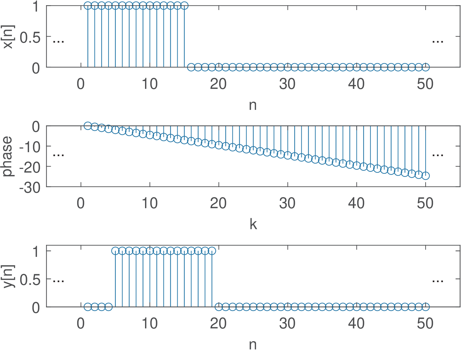
Example 3.13. Impact of the system phase on the output signal. To help understanding the practical importance of a system with linear phase, it is adopted a periodic pulse $x [n]$ with $N_{1} = 15$ (number of non-zero samples in a period) and period $N = 50$ (see Example 2.11). The experiment is to obtain $Y [k]$ by multiplying the DTFS $X [k]$ of $x [n]$ by $e^{- j 2 π N_{0} k ∕ N}$ , where $N_{0} = 4$ . Listing 3.10 carries out the operation, including the conversion of $Y [k]$ to $y [n]$ .

Listing 3.10: MatlabOctaveCodeSnippets/snip_systems_linear_phase_system.m. [ Python version]

1%Specify: N-period, N1/N-duty cicle, N0-delay, k-frequency 
2N=50; N1=15; N0=4; k=0:N-1; 
3xn=[ones(1,N1) zeros(1,N-N1)]; %x[n] 
4Xk=fft(xn)/N; %calculate the DTFS of x[n] 
5phase = -2*pi/N*N0*k; %define linear phase 
6Yk=Xk.*exp(j*phase); %impose the linear phase 
7yn=ifft(Yk)*N; %recover signal in time domain

Figure 3.16 illustrates the result: $y [n] = x [n - N_{0}]$ is a perfect delayed version of $x [n]$ . The middle plot shows the phase that was added to the original phase of $X [k]$ . The magnitude of $X [k]$ was left unchanged but that would not be enough to keep the shape of $x [n]$ in case the phase was not linear with frequency.

Figure 3.16: Effect of adding a linear phase $e^{- j 2 π N_{0} k ∕ N}$ ( $N_{0} = 4$ and $N = 50$ ) to the DTFS of $x [n]$ resulting in a delayed version $y [n] = x [n - 4]$ .

To be contrasted with the linear phase case, Figure 3.17 provides an example where the phase is 0, 2 or $- 2$ rad, as depicted in the top-most plot. In order to assure that $y [n]$ is real, the phase is an odd function to preserve the Hermitian symmetry.

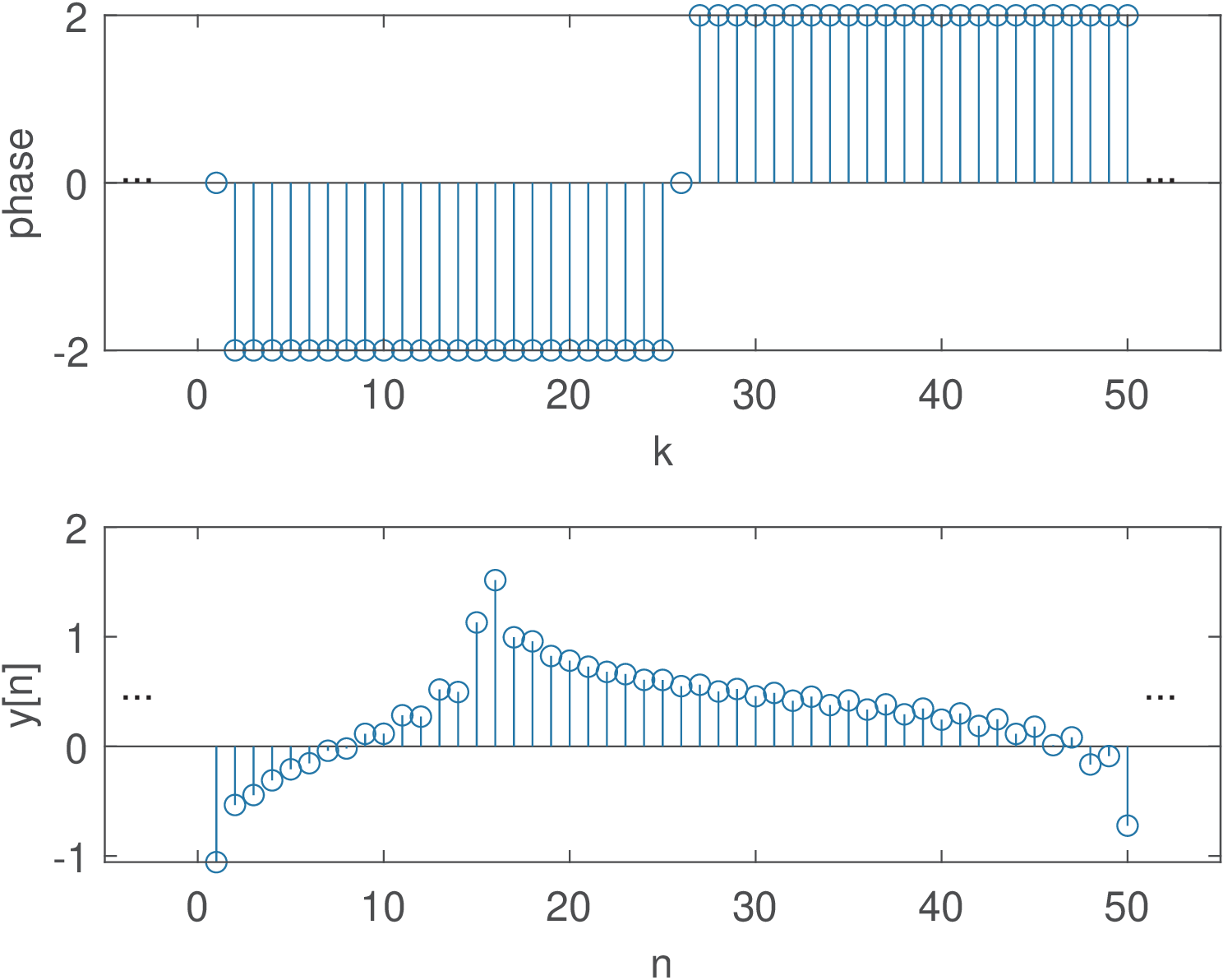
Figure 3.17: Effect of adding the specified nonlinear phase (top) to the pulse in Figure 3.16, which leads to a distorted signal (bottom).

Note that in the case of Figure 3.17, the pulses in $x [n]$ are severely distorted due to the effect of a non-linear phase. $□$

Considering continuous-time (same is valid for discrete-time), a linear phase $e^{- j 2 πf t_{0}}$ avoids distorting an input signal $x (t)$ because the system delays all components of $x (t)$ by the same time interval $t_{0}$ . To obtain that, a linear phase system adds to the input signal component with frequency $f_{i}$ , a phase $Θ_{i} = - 2 π f_{i} t_{0}$ that is proportional to $f_{i}$ (the larger $f_{i}$ , the larger the phase $Θ_{i}$ added by the system). The following example concerns this aspect.

Example 3.14. A linear phase allows components with distinct frequencies to be delayed by the same angle. For example, assume components corresponding to $ω = 200$ and 400 rad/s with $t_{0} = 4$ s. The phases $Θ = ω t_{0}$ are 800 and 1600 rad, respectively. On the other hand, if these two components pass a system that adds a fixed phase $Θ = 1200$ rad to both, the delays would be 6 and 3 s, respectively, which would potentially distort the delayed version with respect to the original signal $x (t)$ . $□$

For non-linear phase filters, the group delay must be interpreted as an average delay that is frequency-dependent (compare Figure 3.55 and Figure 3.56).⁸

Example 3.15. Gaussian filter and minimum group delay. In some applications, such as digital communications, minimizing the group delay is important to achieve low latency. In this case, the Gaussian filter is competitive because it has the minimum possible group delay. As a consequence, this filter has no overshoot to an input $u (t)$ while minimizing the rise and fall time intervals. Its ideal and non-causal impulse response is

h (t) = \frac{\sqrt{π}}{α} e^{- {(\frac{πt}{α})}^{2}},

(3.36)

where $α$ controls the 3-dB bandwidth BW. This $h (t)$ requires truncation in practice.

More specifically, $α$ depends on the product of BW and the symbol period $T_{sym}$ as follows:

α = \frac{1}{BW T_{sym}} \sqrt{\frac{ln 2}{2}} .

(3.37)

The frequency response of this filter is $H (f) = e^{- α^{2} f^{2}}$ and decreases with $f$ but is not zero for finite $f$ . $□$

3.4.8 Filter masks

The filter designer often has a specification mask that should be obeyed. The passband and other special frequencies are used to describe the mask.

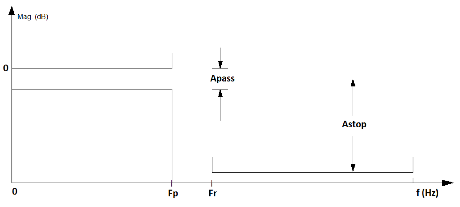
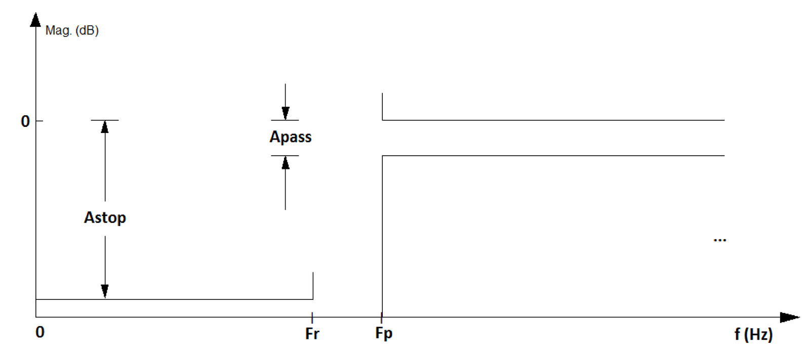
Figure 3.17a and Figure 3.17b depict masks for low and highpass filters, respectively. In this case, the values Apass and Astop indicate the maximum and minimum attenuation in dB for the passband and stopband, respectively. These bands are indicated by the frequencies Fp and Fr, for pass and rejection bands.

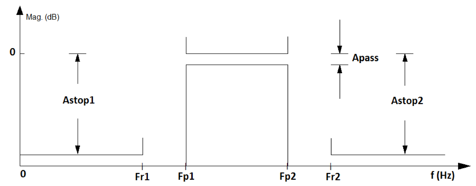
Figure 3.19: Example of specification mask for designing bandpass filters.

Besides lowpass and highpass, some other popular filters are the so-called bandpass and bandstop (or band-reject) filters. Figure 3.19 shows a bandpass specification.

The goal of this section was to provide an overview of filtering. Appendix B.7 presents a brief review of the most important properties of systems and the next section discusses LTI systems.

3.4.9 Designing simple filters using specialized software

Before studying digital filters in more details, it is useful to briefly discuss analog filters because most of the times they are required in digital signal processing systems as will be discussed here.

Example of analog filter design

There are integrated circuits (IC) that implement analog filters. They can also be built using discrete components: resistors, capacitors, inductors and operational amplifiers (opamps). The design of a filter corresponds to obtaining its system function. In the case of analog filters, there are many recipes (well-established algorithms, also called approximations) to obtain a system function $H (s)$ that obeys the specified requirements in a project. The most common approximations are the Butterworth, Chebyshev, Bessel and Cauer (or elliptic).

Having $H (s)$ , the next step is the realization of the filter using a circuit, i. e., establishing the topology and the components of the circuit that (approximately) implement $H (s)$ . These two steps are the subject of many textbooks on filter design. Here, the approach will be to simply provide an example using software from Texas Instruments [ url3tif] that allows to obtain the schematic and components.⁹

Analog filters that use only resistor, capacitors and inductors are called passive filters. An alternative to avoid using inductors¹⁰ are active filters, which are typically based on opamps. When the target is an IC, not a circuit with discrete components, inductors are avoided due to the difficulty of their integration using current microelectronics technology. When an analog filtering operation is required in an IC, an active filter is typically adopted and this is the only class of filters supported by the mentioned Texas Instruments’ software.

Example 3.16. Example of analog filter designed with Texas Instruments’ software. The following example illustrates the design of an analog filter with a desired cutoff frequency $f_{c} = 1$ kHz, which is assumed to define the passband, such that the passband frequency is $f_{p} = f_{c}$ . A second-order lowpass filter with passband frequency of approximately $996.7678$ Hz was obtained with Texas Instruments’ software and its schematic¹¹ is shown in Figure 3.20.

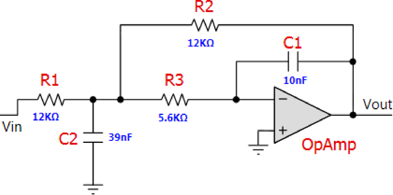
Figure 3.20: Lowpass active analog filter designed with Texas Instruments’ software.

The system function $H (s)$ can be obtained by analyzing the circuit in Figure 3.20 and is given by

H (s) = \frac{V_{out} (s)}{V_{signal} (s)} = - \frac{R_{2} ∕ R_{1}}{s^{2} R_{2} R_{3} C_{1} C_{2} + s C_{1} R_{2} R_{3} (\frac{1}{R_{1}} + \frac{1}{R_{2}} + \frac{1}{R_{3}}) + 1},

(3.38)

where the suffix “_S1” (meaning “stage 1”) was removed from the names of the components in Figure 3.20. For instance, $R_{2}$ in Eq. (3.38) corresponds to R2_S1 in Figure 3.20. Note the minus signal in $H (s)$ of Eq. (3.38) because the circuit corresponds to an inverting topology.

Substituting the component values $R_{1} = R_{2} = 10.5 k Ω$ , $R_{3} = 6.04 k Ω$ , $C_{1} = 10 nF$ and $C_{2} = 40.2 nF$ into Eq. (3.38) yields

H (s) = - \frac{1}{2.5519 \times 1 0^{- 8} s^{2} + 2.2575 \times 1 0^{- 4} s + 1} = - \frac{3.9187 \times 1 0^{7}}{s^{2} + 8.8469 \times 1 0^{3} s + 3.9187 \times 1 0^{7}},

Rearranging the denominator into the standard second-order form,

H (s) = - \frac{3.9187 \times 1 0^{7}}{s^{2} + 8.8469 \times 1 0^{3} s + 3.9187 \times 1 0^{7}},

which has a cutoff frequency $f_{c} = 996.7678$ Hz.¹²

The ideal system function can be obtained e. g. with Matlab/Octave via the command: [Bs,As]=butter(2,2*pi*1000,’s’) that gives

H (s) = \frac{B (s)}{A (s)} = \frac{3.9478 \times 1 0^{7}}{s^{2} + 8.8858 \times 1 0^{3} s + 3.9478 \times 1 0^{7}} .

(3.39)

The arguments of the function butter are the filter order and the cutoff frequency in rad/s (not Hz). Note the required ’s’ to indicate to Matlab/Octave that the goal is to design an analog, not a digital filter.

To obtain Eq. (3.39), one can choose the values $C_{1} = 10 nF$ and $C_{2} = 40 nF$ , and then $R_{1} = R_{2} = 11.25395 k Ω$ and $R_{3} = 5.62698 k Ω$ . In this case, the cutoff frequency $f_{c}$ would be exactly 1 kHz. But conventional resistors do not have exactly these resistance values. In practice, commercial components are available only within a finite set of values and their actual values differ from the nominal ones, according to a given non-zero tolerance (e. g., 2% or 10%). $□$

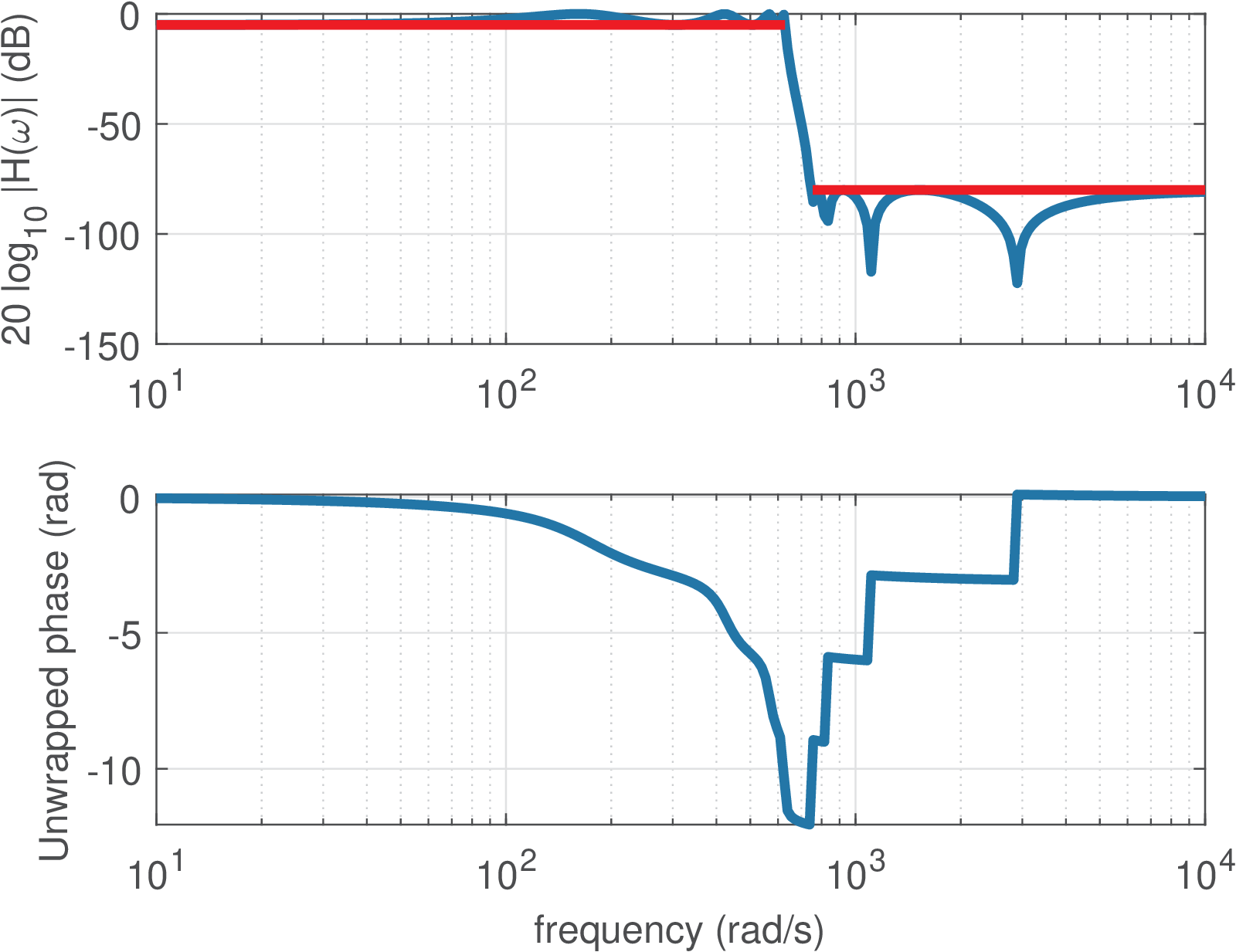
Example 3.17. Further examples of analog filter design in Matlab. Listing 3.11 illustrates how to design some analog filters with a given specification for its magnitude using Matlab (this code is not compatible with Octave). The frequency response magnitude and phase of the four designed filters are depicted in Figure 3.21.

Listing 3.11: MatlabBookFigures/figs_systems_elliptic.m

1Apass=5; %maximum ripple at passband 
2Astop=80; %minimum attenuation at stopband 
3%% Lowpass Elliptic %%%%%%%%% 
4Fp=100; Wp=2*pi*Fp; %passband frequency 
5Fr=120; Wr=2*pi*Fr; %stopband frequency 
6[N, Wp] = ellipord(Wp, Wr, Apass, Astop, 's') %find order 
7[z,p,k]=ellip(N,Apass,Astop,Wp,'s'); %design filter 
8B=k*poly(z); A=poly(p); %convert zero-poles to transfer function 
9[H,w]=freqs(B,A); %calculate frequency response 
10%% Higpass Elliptic %%%%%%%%% 
11Fr=100; Wr=2*pi*Fr; %stopband frequency 
12Fp=120; Wp=2*pi*Fp; %passband frequency 
13[N, Wp] = ellipord(Wp, Wr, Apass, Astop, 's') %find order 
14[z,p,k]=ellip(N,Apass,Astop,Wp,'high','s'); %design filter 
15B=k*poly(z); A=poly(p); %convert zero-pole to transfer function 
16[H,w]=freqs(B,A); %calculate frequency response 
17%% Bandpass Elliptic %%%%%%%% 
18Fr1=10; Wr1=2*pi*Fr1; %first stopband frequency 
19Fp1=20; Wp1=2*pi*Fp1; %first passband frequency 
20Fp2=120; Wp2=2*pi*Fp2; %second passband frequency 
21Fr2=140; Wr2=2*pi*Fr2; %second stopband frequency 
22[N,Wp]=ellipord([Wp1 Wp2],[Wr1 Wr2],Apass,Astop,'s') %find order 
23[z,p,k]=ellip(N,Apass,Astop,Wp,'s');%design filter 
24B=k*poly(z); A=poly(p); %convert zero-pole to transfer function 
25[H,w]=freqs(B,A); %calculate frequency response 
26%% Bandpass Butterworth %%%%%%%%%%% 
27[N, Wn]=buttord([Wp1 Wp2],[Wr1 Wr2],Apass,Astop,'s')%find order 
28[z,p,k]=butter(N,Wn,'s'); %design Butterworth filter 
29B=k*poly(z); A=poly(p); %convert zero-pole to transfer function 
30[H,w]=freqs(B,A); %calculate frequency response

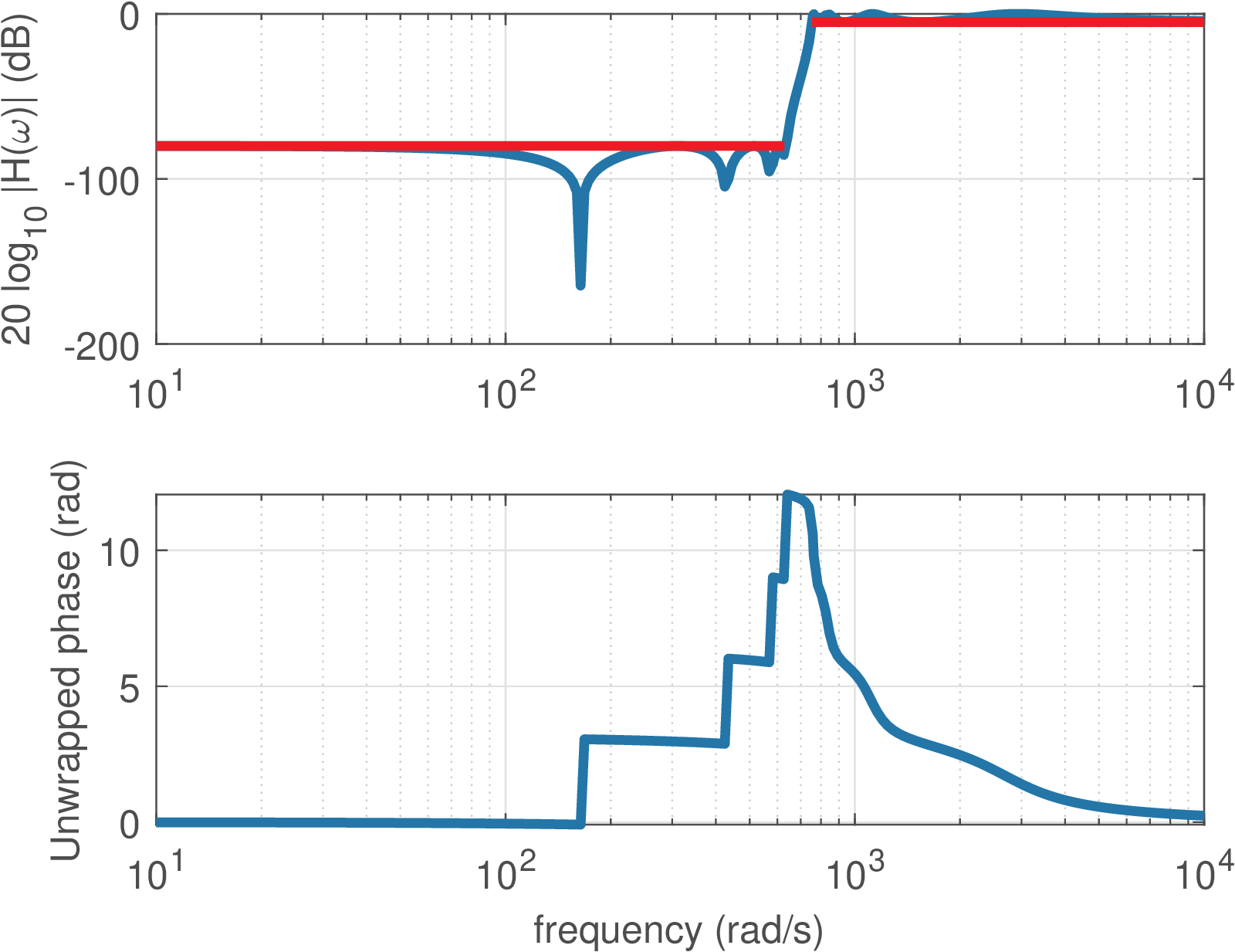
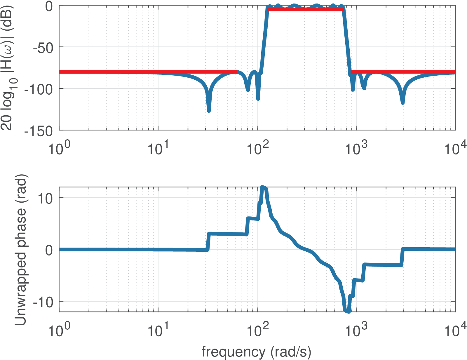
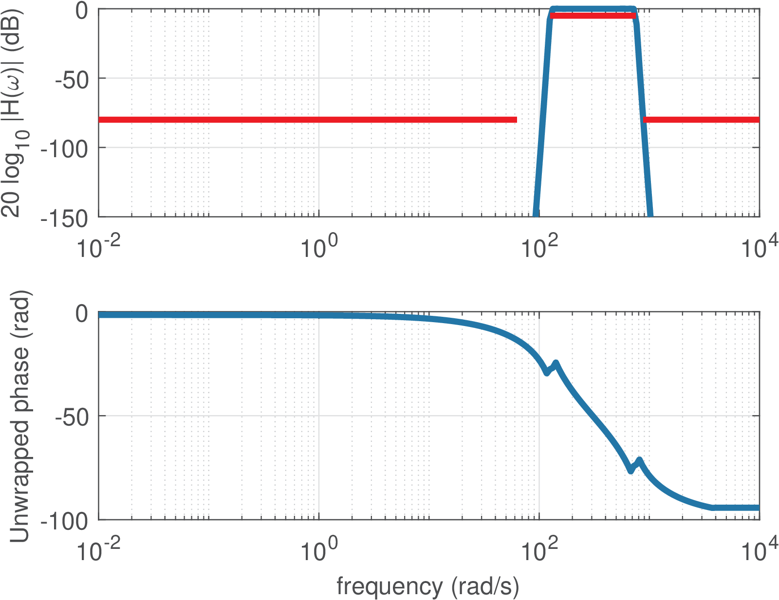
It should be noted from Listing 3.11 and Figure 3.21 that a bandpass filter has twice the order that is specified as an input parameter (and obtained by buttord and ellipord in this example). Note also that, in practice, an analog filter typically has an order between 1 to 10. For example, an order $N = 86$ is not feasible for practical implementation with an analog circuit. $□$

Example of digital filter design

Figure 3.22: The canonical interface of a digital filter $H (z)$ with the analog world via ADC and DAC chips. The analog $A (s)$ and $R (s)$ are the anti-aliasing and external reconstruction filters, respectively.

For comparison, it is interesting to design now an equivalent digital filter $H (z)$ to substitute its analog counterpart corresponding to $H (s)$ . But in order to interface $H (z)$ with the external (analog) world, four extra blocks are required, as illustrated in Figure 3.22. The filters $A (s)$ (anti-aliasing) and $R (s)$ (external reconstruction) are lowpass analog filters with passband frequency equal to half of the sampling frequency, which is assumed here to be $F_{s} = 10$ kHz. Their gains are not important at this moment and in practice they are determined by the interfacing electronics. Assuming the converters and analog filters are properly defined, it remains to design $H (z)$ , which can be done with the command

1[Bz,Az]=butter(2,(1000/5000))

that leads to

H (z) = \frac{B (z)}{A (z)} = \frac{0.067455 + 0.134911 z^{- 1} + 0.067455 z^{- 2}}{1.0 - 1.14298 z^{- 1} + 0.41280 z^{- 2}} .

(3.40)

It is important to note that when designing an analog filter, the second argument of butter is $ω$ in rad/s. For a digital filter, as explained in Section 1.8.4, Matlab/Octave uses the normalized frequency $f_{N} = Ω ∕ π$ . In this case, the Nyquist frequency $F_{s} ∕ 2$ is 5 kHz and using Eq. (1.39), $f = 1000$ Hz is normalized by the Nyquist frequency in the command [Bz,Az]=butter(2,(1000/5000)).

It will be later discussed in this chapter that the function butter used the bilinear transformation to convert $H (s)$ of Eq. (3.39) into $H (z)$ of Eq. (3.40).

From Table 3.1 one knows the definition $H (z) = Y (z) ∕ X (z)$ and this should not be confused with $H (z) = B (z) ∕ A (z)$ in Eq. (3.40). In many applications $H (z)$ is a rational function (a ratio of two polynomials), with $B (z)$ specifying the numerator and $A (z)$ the denominator. In general, $B (z) \neq Y (z)$ and $A (z) \neq X (z)$ .

Digital filters described by a rational function $H (z)$ can be conveniently implemented via a LCCDE, as discussed next.

Example 3.18. Obtaining the difference equation and implementing a digital filter. For example, assume that a LTI system with impulse response $h [n] = 0 . 2^{n} u [n]$ outputs $y [n] = δ [n] - 0.3 δ [n - 1]$ when the input is $x [n] = δ [n] - 0.5 δ [n - 1] + 0.06 δ [n - 2]$ . In this case, $X (z) = 1 - 0.5 z^{- 1} + 0.06 z^{- 2}$ and $Y (z) = 1 - 0.3 z^{- 1}$ , which leads to $H (z) = 1 ∕ (1 - 0.2 z^{- 1})$ with $B (z) = 1$ and $A (z) = 1 - 0.2 z^{- 1}$ . With this concept in mind, Eq. (3.40) can be written as

\begin{array}{l} X (z) (0.067455 + 0.134911 z^{- 1} + 0.067455 z^{- 2}) \\ = Y (z) (1.0 - 1.14298 z^{- 1} + 0.41280 z^{- 2}) \end{array}

and taking the Z-inverse one can obtain the difference equation corresponding to Eq. (3.40):

\begin{array}{l} y [n] & = 0.067455 x [n] + 0.134911 x [n - 1] + 0.067455 x [n - 2] \\ + 1.14298 y [n - 1] - 0.41280 y [n - 2] . \end{array}

The amazing fact is that this can be implemented with a simple code, similar to Listing 3.12.

Listing 3.12: Digital filter implementation in pseudo-code.

1initialization() { %all previous values are assumed 0 
2    xnm1=0 %variable to store the value of x[n-1] 
3    xnm2=0 %x[n-2] 
4    ynm1=0 %y[n-1] 
5    ynm2=0 %y[n-2] 
6} 
7processSample() { 
8    xn=readFromADConverter() %read input sample from ADC 
9    yn=0.067455*xn + 0.134911*xnm1 + 0.067455*xnm2 + 
10       1.14298 ynm1 - 0.41280 *ynm2 
11    writeToDAConverter(yn) %write output sample into DAC 
12    ynm2=ynm1 %update for next iteration. Note the order of ... 
13    ynm1=yn   %updates: avoid overwriting a value ... 
14    xnm2=xnm1 %that should be used later 
15    xnm1=xn 
16}

where one assumes a timer¹³ invokes the function processSample at a rate of $F_{s}$ (10 kHz in this case).

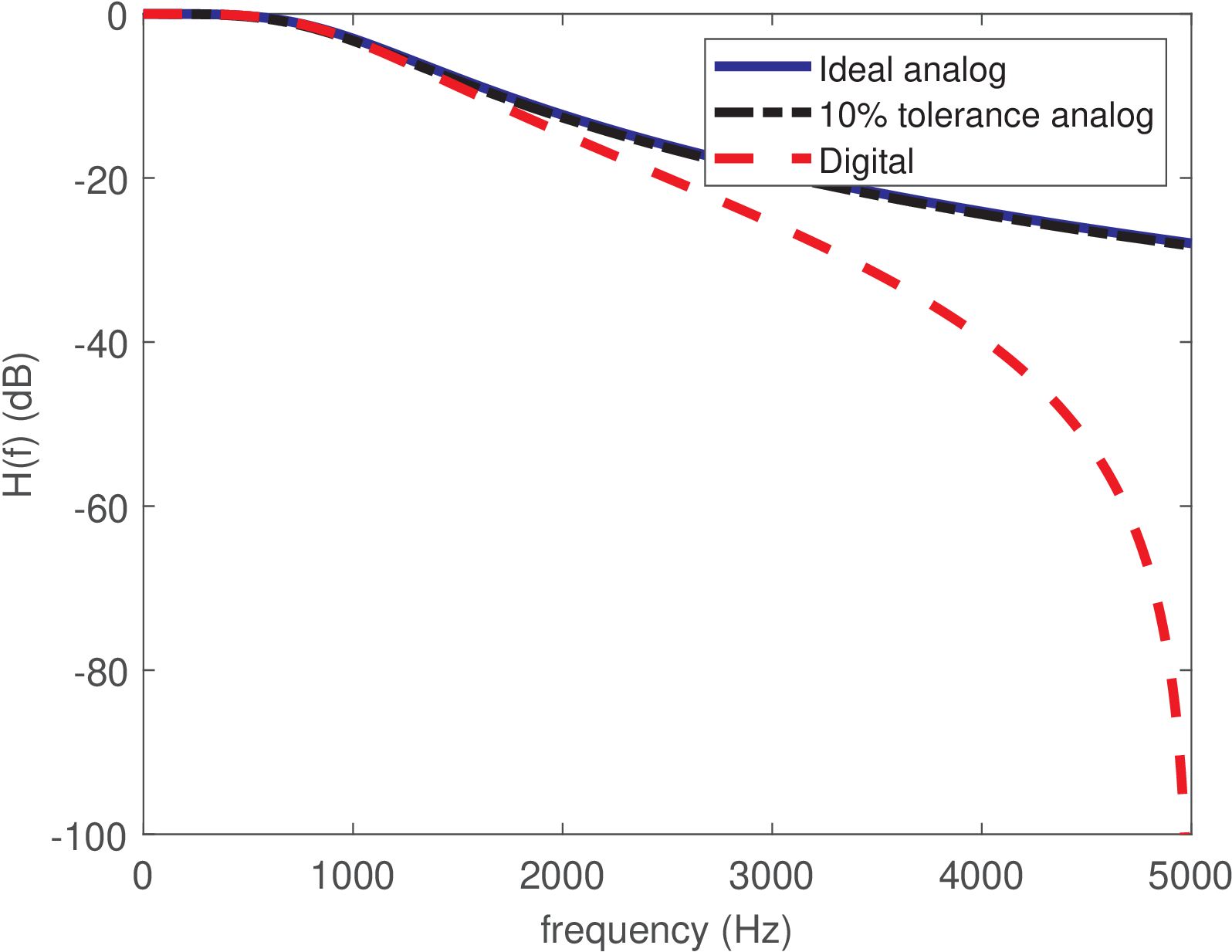
Figure 3.23: Comparison of two analog filters with its digital counterpart of Eq. (3.40). The “ideal” analog corresponds to Eq. (3.39) while the “10% tolerance” corresponds to its realization using the schematic of Figure 3.20.

Figure 3.23 compares the discussed filters, illustrating that $H (z)$ has a lowpass frequency response that is similar in terms of passband frequency to the original $H (s)$ . For frequencies above the passband, $H (z)$ attenuates more than $H (s)$ , but this is not deleterious for a lowpass filter. Later, in Section 3.8.4, this behavior will be clarified, which is intrinsic of having the bilinear transformation mapping the behavior of the analog filter at infinite frequencies into $Ω = π$ rad (or $F_{s} ∕ 2$ Hz) for $H (z)$ , i. e., mapping $H (ω) |_{ω \to \infty}$ into $H (e^{j Ω}) |_{Ω = π}$ .

If $F_{s}$ is changed, the frequency response of the overall system in Figure 3.22 is scaled according to $ω = Ω F_{s}$ (Eq. (1.35)). For example, decreasing $F_{s}$ from 10 to 5 kHz would divide by two the cutoff frequency of the overall system. $□$

3.4.10 Distinct ways of specifying the “ripple” deviation in filter design

As illustrated in Figure 3.21, practical filters have a frequency response that deviates from the ideal ones. Instead of a flat magnitude over the whole passband and zero gain in the stopband, as depicted in Figure 3.8, a non-ideal filter has deviations from the target values and eventual “oscillations” called “ripples”. When designing a filter, it is possible to impose limits to these ripples, but this procedure is different for the passband and stopband “ripples” / deviations, as discussed next.

There are several ways of specifying the maximum “ripple” or deviation at the passband of a filter. For example, it can be specified in dB or linear scale, which are called here $R_{p}$ and $D_{p}$ , respectively (as suggested by Matlab). If one assumes a lowpass filter with a unitary gain at DC, the maximum linear deviation $D_{p}$ can be assumed to be within $[1 - D_{p}, 1 + D_{p}]$ or $[1 - D_{p}, 1]$ . The latter option is particularly useful if the filter magnitude monotonically decreases as for the Butterworth filters and is assumed here, meaning that the frequency response is 1 at DC and decreases in the passband to a value not smaller than $1 - D_{p}$ . For example, a specification can be that the passband magnitude does not deviate 5% of the gain at DC. In this case, $D_{p} = 0.05$ and the minimum magnitude at passband is $1 - D_{p} = 0.95$ . Often, this value is specified in dB as

R_{p} = - 20 \log_{10} (1 - D_{p}) .

If the deviation is within $[1 - D_{p}, 1]$ in linear scale, then it is confined to $[- R_{p}, 0]$ in dB.

At the stopband, the magnitude in linear scale $D_{s}$ is also a “deviation” because the reference value is 0 (the desired magnitude at stopband). In other words, for the stopband, the deviation coincides with the magnitude itself and its value in dB is given by

R_{s} = - 20 \log_{10} D_{s} .

Often, the filter magnitude has a maximum value of 0 dB and the values of $R_{p}$ and $R_{s}$ are positive.

Matlab uses the same convention adopted here in its routines. This is exemplified in Listing 3.13, which uses the method buttord to find the order of a Butterworth filter that complies with the project specifications.

Listing 3.13: MatlabOctaveCodeSnippets/snip_systems_IIR_design.m. [ Python version]

1Wp=0.3; %normalized passband frequency (rad / pi) 
2Ws=0.7; %normalized stopband frequency (rad / pi) 
3Rp=1; %maximum passband ripple in dB 
4Rs=40; %minimum stopband attenuation in dB 
5[n,Wn] = buttord(Wp,Ws,Rp,Rs); %find the Butterworth order 
6[B,A]=butter(n,Wn); %design the Butterworth filter 
7zp=exp(1j*pi*Wp); zs=exp(1j*pi*Ws); %Z values at Wp and Ws 
8%% Check if the filter obeys requirements 
9linearMagWp = abs(polyval(B,zp)/polyval(A,zp)) %mag. at Wp 
10linearMagWs = abs(polyval(B,zs)/polyval(A,zs)) %mag. at Ws 
11Dp_result = 1-linearMagWp %linear deviation at Wp (linear) 
12Rp_result = -20*log10(1-Dp_result) %deviation (ripple) at Wp (dB) 
13Ds_result = linearMagWs %linear deviation at Ws (linear) 
14Rs_result = -20*log10(Ds_result) %deviation (ripple) at Ws (dB)

The required filter order is n=4, and the obtained results are: linearMagWp=0.9105, linearMagWs=0.01, Dp_result=0.0895, Rp_result=0.8147, Ds_result=0.01 and Rs_result=40.0. They can be interpreted as follows. Matlab designed the method buttord to meet exactly the requirements for the stopband, while giving an eventual slack to the requirements for the passband. Hence, we can see that Rs_result=40.0 dB is exactly the specified attenuation at the stopband. This corresponds to a linear gain linearMagWs=0.01 of the filter’s frequency response $H (e^{j Ω})$ at the beginning of the stopband. Using mathematical notation: $H (e^{j Ω}) |_{Ω = 0.7 π} = 0.01$ in linear scale, which corresponds to $20 \log_{10} H (e^{j Ω}) |_{Ω = 0.7 π} = 20 \log_{10} (0.01) = - 40$ dB.

The filter gain is 1 at DC, and it decreases until reaching linearMagWp=0.9105 in the end of its passband. In our notation, $H (e^{j Ω}) |_{Ω = 0.3 π} = 0.9105$ , which corresponds to $20 \log_{10} H (e^{j Ω}) |_{Ω = 0.3 π} = 20 \log_{10} (0.9105) = - 0.8144$ dB. This value does not coincide with Rp_result=0.8147 due to the rounding to four decimal places. Using 20*log10(linearMagWp) gives the precise gain value of $- 0.8147$ dB. Note that the deviation in the passband of 0.8147 dB from the ideal 0 dB is within the maximum value of 1 dB imposed to buttord. There is a slack of $1 - 0.8147 = 0.1853$ dB.

In summary, it is a bit confusing how Matlab and other software define the input parameters to functions such as buttord. But one just needs to interpret the ripples in dB as obtained from “deviations” of the ideal values of 1 and 0 in passband and stopband, respectively.

3.4.11 LCCDE digital filters

A digital filter is a discrete-time system that deals with quantized input $x_{q} [n]$ and output $y_{q} [n]$ signals (quantized amplitudes). A possible practical scenario for a digital filter is the one shown in Figure 3.22. There are many different kinds of digital filters but this section assumes filters that are based on linear constant-coefficient difference equations (LCCDE). As indicated in Figure 3.1, when zero initial conditions are assumed, the LCCDE systems are a special case of LTI systems. But when one takes in account the non-linear quantization effects that occur in practical CPUs (or digital signal processors) due to their limited precision, the overall system is not strictly LTI. In spite of that, it is convenient to isolate the effects of quantization and finite-precision arithmetics, and study digital filters as LTI LCCDE systems. Later on, the impact of quantizing the filter coefficients and the roundoff errors due to finite-precision can be incorporated. Therefore, hereafter, the term digital filter refers to discrete-time LTI LCCDE systems. Besides, the systems are assumed to be causal.

A system that has the output and input signals related by a LCCDE such as

\sum_{k = 0}^{N} a_{k} y [n - k] = \sum_{k = 0}^{M} b_{k} x [n - k]

(3.41)

can be represented by (taking the Z-transform on both sides of the LCCDE)

Y (z) \sum_{k = 0}^{N} a_{k} z^{- k} = X (z) ∑_{k = 0}^{M} b_{k} z^{- k} .

In this case, the transfer function is

H (z) = \frac{Y (z)}{X (z)} = \frac{\sum_{k = 0}^{M} b_{k} z^{- k}}{\sum_{k = 0}^{N} a_{k} z^{- k}},

(3.42)

which, after eventual algebraic simplifications, can be written as the ratio

H (z) = \frac{B (z)}{A (z)}

(3.43)

of two polynomials in $z$ . Calculating the zeros $z_{k}$ (roots of the numerator $B (z)$ ) and the poles $p_{k}$ (roots of the denominator $A (z)$ ), one can write

H (z) = g \frac{\prod_{k = 1}^{M} (z - z_{k})}{\prod_{k = 1}^{N} (z - p_{k})},

where $g$ is a gain. The coefficients of Eq. (3.41) can be real or complex. For simplicity, they will be assumed real ( $a_{k}, b_{k} \in ℝ$ ) unless otherwise stated. In this case, $g \in ℝ$ and the roots $z_{k}, p_{k}$ are real or, for each root $r e^{j𝜃}$ , its complex conjugate $r e^{- j𝜃}$ is also a root such that the product $(z - r e^{j𝜃}) (z - r e^{- j𝜃}) = z^{2} + 2 r cos (𝜃) + r^{2}$ leads to a second-order polynomial with real coefficients.

It is useful to know that the value of $H (z)$ at $z = 1$ and $z = - 1$ correspond to the values of the frequency response $H (e^{j Ω})$ at $Ω = 0$ (DC) and $Ω = π$ rad, respectively, which can be written as

H (z) |_{z = 1} = H (e^{j Ω}) |_{Ω = 0} and H (z) |_{z = - 1} = H (e^{j Ω}) |_{Ω = π} .

(3.44)

For example $H (z) = 3 + z^{- 1}$ has a frequency response with $H (e^{j Ω}) |_{Ω = 0} = 3 + 1 = 4$ and $H (e^{j Ω}) |_{Ω = π} = 3 - 1 = 2$ .

Example 3.19. Specifying a filter in Hz, rad or normalized frequency. When designing digital filters, it is important to remember the fundamental relation $ω = Ω F_{s}$ , first presented in Eq. (1.35). Figure 3.24 illustrates how this relation can be used to convert a specification for a lowpass analog filter with passband and stopband frequencies of 500 and 850 Hz, respectively, into a specification of a digital filter with $F_{s} = 2000 Hz$ , which leads to passband and stopband frequencies of $2 π 500 ∕ 2000 \approx 1.57$ and $2 π 850 ∕ 2000 \approx 2.67$ rad, respectively.

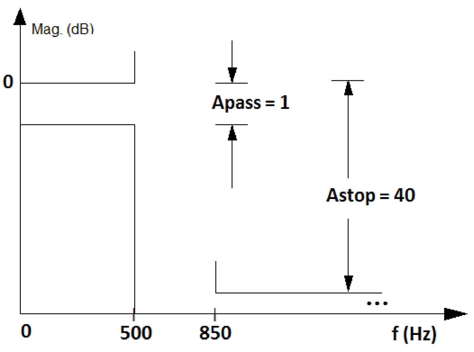
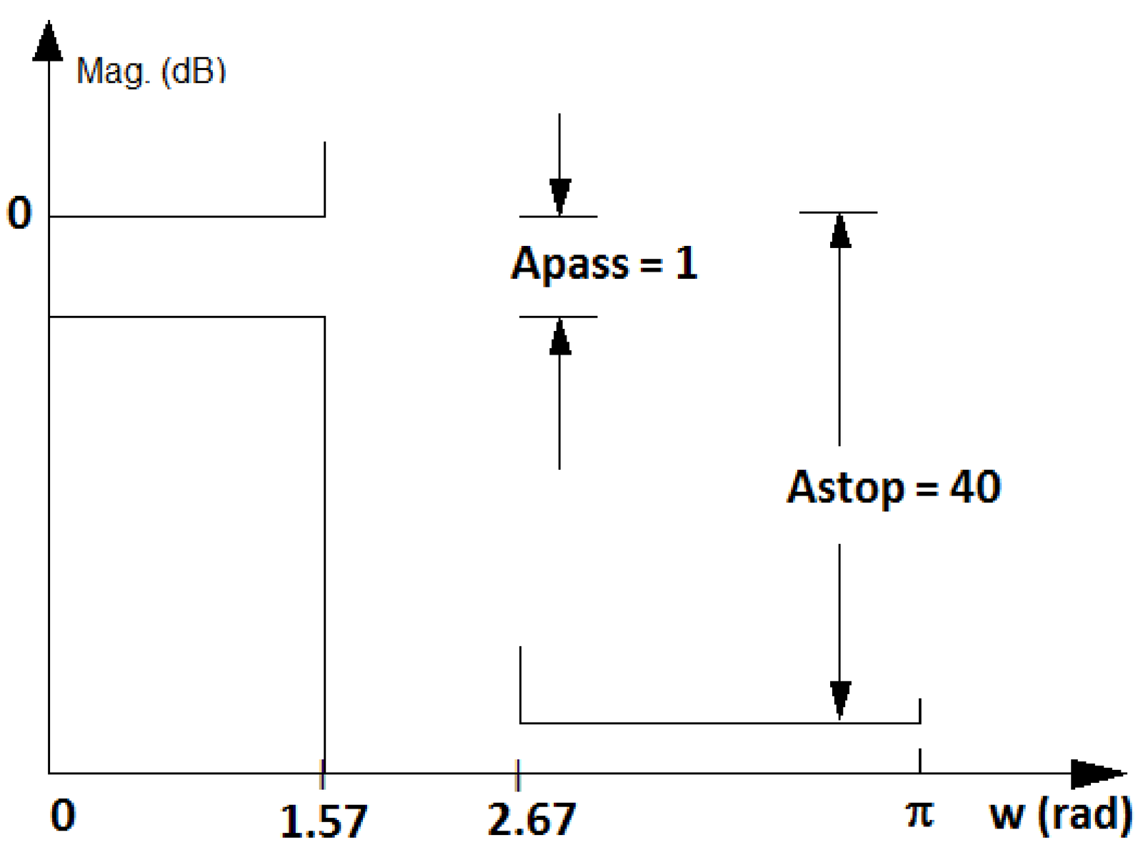
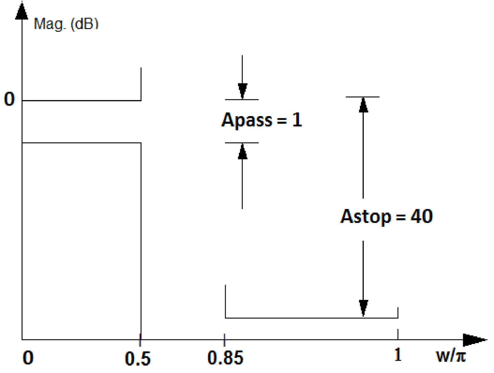
Figure 3.24 also shows the convention used by Matlab/Octave, which gets rid of the irrational number $π$ by using a normalized axis $f_{N} = Ω ∕ π$ , as listed in Table 1.5. In this case, $ω = Ω F_{s}$ can be written as $2 πf = f_{N} π F_{s}$ , which simplifies to obtaining $f_{N} = f ∕ (F_{s} ∕ 2)$ with the normalization of $f$ by the Nyquist frequency $F_{s} ∕ 2$ . For example, $f = 500$ Hz in Figure 3.23a turns into $f_{N} = 500 ∕ 1000 = 0.5$ in Figure 3.23c. This normalization by the Nyquist frequency is sensible because digital filters are always constrained to work with frequencies of at most $F_{s} ∕ 2$ Hz, which corresponds to $π$ rad. $□$

3.4.12 Advanced: Surface acoustic wave (SAW) and other filters

There are several technologies to build an electronic filter. The options include ceramic, microelectromechanical system (MEMS), yttrium iron garnet (YIG), SAW and many others. Even if the scope is reduced to radio-frequency (RF) communications, the diversity of filters is huge. Consequently, parameters such as the Q-factor, center frequency $f_{c}$ and insertion loss. This section provides some practical examples.

Example 3.20. Performance of commercial SAW filter. Figure 3.25 illustrates the typical performance of a commercial SAW filter¹⁴ with some of its specifications listed in Table 3.5. The insertion gain $IG (f)$ is shown in Figure 3.25 at 1 and 10 dB per division (div) at the left plot and superimposed (at 1 dB per division) to the group delay at the right plot.

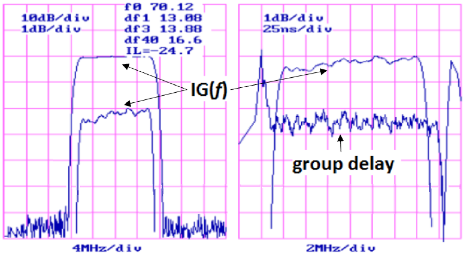
Figure 3.25: Performance of a commercial SAW filter. The insertion gain $IG (f)$ at two resolutions at the left plot and superimposed to the group delay at the right.

As also indicated in Table 3.5, Figure 3.25 indicates that df1, df3 and df40 are the bandwidths considering the attenuation at 1, 3 and 40 dB, respectively, with values 13.08, 13.88 and 16.6 MHz. The insertion loss $IL (f) |_{f = f_{c}}$ at $f_{c} = 70.12$ MHz is 24.7 dB. The group delay plot only shows the variation at the order of ns, but Table 3.5 indicates the delay as 1.6 $μ$ s. $IG (f)$ is sometimes called IL and Figure 3.25 uses a negative IL to express that the filter attenuates the power by 24.7 dB as properly expressed in Table 3.5.

Table 3.5: Specifications of a commercial SAW filter.


Parameter	Minimum	Typical	Maximum

Center frequency at $2 5^{o}$ C ( $f_{c}$ or f0, MHz)	69.8	70	70.2

Insertion loss at $f_{c}$ (IL, dB)	-	24.7	28.0

1-dB bandwidth (df1, MHz)	12.75	13.0	-

3-dB bandwidth (df3, MHz)	13.0	13.8	-

40-dB bandwidth (df40, MHz)	-	16.6	17.1

Passband variation (ripple, dB)	-	0.5	0.6

Group delay variation (ns)	-	25	50

Absolute delay ( $μ$ s)	-	1.6	-

The Q-factor of the filter depicted in Figure 3.25 is $Q = 70.12 ∕ 13.88 \approx 5$ and provides more than 60 dB of attenuation at the stopband. Building such (relatively) highly-selective filters is easier when the center frequency $f_{c}$ is fixed than when it has to vary, for tuning purposes. For example, the filter of Figure 3.25 is supposed to operate with $f_{c} = 70$ MHz, which is an intermediate frequency (IF) used in wireless signal reception. When a receiver has to operate over a frequency range, a common strategy is to pre-select the frequency band of interest using a so-called RF-filter with center frequency $f_{c}^{RF}$ (e. g., 2.1 GHz) and convert it via frequency shifting to the IF (e. g., 70 MHz), when it is then better filtered and further processed. $□$

A common IF for broadcast AM radio is $f_{c} = 455$ kHz, which motivates the next filter example.

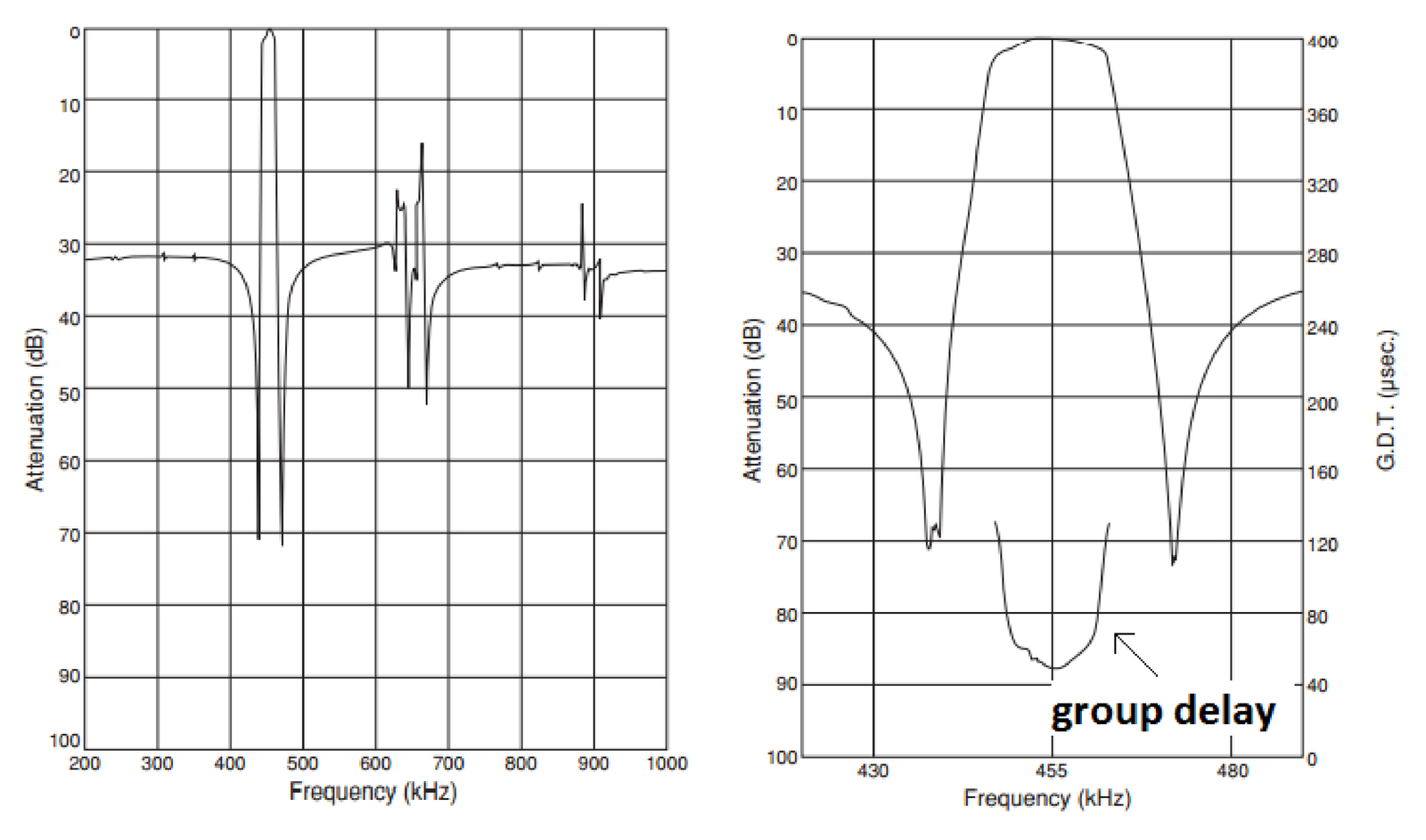
Example 3.21. Commercial ceramic filter. Figure 3.26 illustrates the performance of a commercial ceramic filter¹⁵ that can be used with an IF of 455 kHz and has some specifications listed in Table 3.6. Note that this filter’s stopband is not flat, especially within the range from 600 to 700 kHz. This makes the specifications harder to interpret than for an ideal bandpass filter.

Figure 3.26: Performance of a commercial ceramic filter. The right plot is a zoom of the attenuation at the left plot, centered at $f_{c} = 455$ kHz and includes the group delay with values ranging between approximately 50 and 120 $μ$ s in passband.

Table 3.6: Specifications of a commercial ceramic filter where

f_{n} = 455

kHz is the nominal frequency and

f_{c}

is the center of the 6-dB BW.


Parameter	Value

Center frequency $f_{c}$ (kHz)	$455 \pm 1.5$

Minimum 6-dB bandwidth (kHz)	$f_{n} \pm 7.5$

Maximum stop bandwidth, within 40 dB (kHz)	$f_{n} \pm 15.0$

Minimum stopband attenuation within $f_{n} \pm 100.0$ kHz (dB)	27

Maximum insertion loss (at minimum loss point, dB)	6

Maximum ripple within $f_{n} \pm 5.0$ kHz (dB)	1.5

Caution has to be exercised when interpreting the “Maximum stop bandwidth” in Table 3.6, which indicates the filter attenuates 40 dB at the end of a band centered on $f_{n}$ and with a bandwidth of approximately 30 kHz. But this attenuation then decreases. According to Table 3.6, an attenuation of at least 27 dB is guaranteed only within $455 \pm 100$ kHz. $□$

3.4.13 FIR, IIR, AR, MA and ARMA systems

An important characteristic of a digital filter is the duration of its impulse response, which allows to classify it as a finite impulse response (FIR) or infinite impulse response (IIR) filter. For example, a filter with $h_{f} [n] = 3 δ [n] + 2 δ [n - 1]$ is FIR and a filter with $h_{i} [n] = 0 . 8^{n} u [n]$ is IIR. Note that if one plots $h_{i} [n]$ in a computer, due to the limited precision, the values of $h_{i} [n]$ would underflow to zero for large enough $n$ , but theoretically this impulse response has infinite duration.

Another characteristic is whether the filter is recursive or not. A recursive filter has the output $y [n]$ depending on past values of the output itself ( $y [n - 1], y [n - 2], \dots$ ) while the output of a non-recursive filter depends only on the input $x [n]$ and its past values (assuming causality). The system function $H (z)$ of a non-recursive filter has $N = 0$ in Eq. (3.42) and no finite poles.

In practice, FIR can be associated to non-recursive filters and IIR to recursive filters. But recursiveness and impulse response duration are two distinct concepts! It is possible to create a recursive filter with an impulse response of finite duration using cancellation of poles and zeros, for example. In spite of that, the design of recursive filters is often called “IIR design”. Similarly, “FIR design” is the topic that concerns the design of non-recursive filters. This widely adopted jargon is used in this text.

IIR and FIR filters will be discussed in the sequel. While the subject is presented in the context of digital filtering, many conclusions are valid for systems in general. In other words, IIR and FIR systems can be found in applications in which the goal is not filtering, but system identification, equalization, control, tracking, statistics, etc. In some of these areas, $H (z)$ is not classified as FIR or IIR, but as MA, AR or ARMA “model”.

A moving-average (MA) model $H (z)$ is a non-recursive FIR filter and an autoregressive (AR) filter is a special case of a recursive IIR filter for which $M = 0$ in Eq. (3.42). The AR IIR filter does not have finite zeros other than at the origin $z = 0$ and is given by

H (z) = g \frac{z^{N}}{\prod_{k = 1}^{N} (z - p_{k})} = \frac{g}{1 + a_{1} z^{- 1} + a_{2} z^{- 2} + \dots + a_{N} z^{- N}} .

(3.45)

Note in Eq. (3.45) that the gain value $g$ for the numerator is chosen such that the denominator coefficient $a_{0}$ of Eq. (3.42) is equal to 1. The numerator $z^{N}$ leads to $N$ zeros at $z = 0$ and makes $H (z)$ causal.

The autoregressive-moving-average (ARMA) model is a generic $H (z)$ model composed by an AR (denominator) and MA (numerator) sections. There are many generalizations of these basic models, which are adopted in areas such as statistics. Parametric modeling is the task of, according to a predefined criterion such as least-squares, fit the data to the assumed model. In spite of being defined in distinct scenarios, filter design and parametric modeling share several fundamental results.

Before discussing the design of IIR and FIR filters, it is useful to note the importance of frequency scaling.

3.4.14 Filter frequency scaling

Computational routines often produce a prototype with normalized frequencies (e. g., a cuttof frequency of 1 rad/s) that are then converted (eventually by another routine) to the required frequencies via frequency scaling.

With frequency scaling one can modify a filter to obtain a different cutoff frequency. For example, if $H (s)$ has a cutoff of $ω_{c}$ rad/s, the transformation $s \to s ∕ k$ moves this cutoff frequency to $k ω_{c}$ rad/s. The operation is similar to using $x (2 t)$ to double the “speed” of a signal represented by $x (t)$ , which leads to $x (2 t)$ having half of the support of $x (t)$ . Similarly, $x (t ∕ 2)$ has twice the support of $x (t)$ . More specifically, if the prototype $H (s)$ has a cutoff frequency of 1 rad/s, then

G (s) = H (s) |_{s = s ∕ ω_{c}}

(3.46)

scales the complex plane, and consequently $s = jω$ , such that $ω_{c}$ is the cutoff frequency of the new filter $G (s)$ .

There are computational routines that provide a prototype filter with (normalized) cutoff frequency of $1$ rad/s, which can then be converted to a new filter with an arbitrary cutoff frequency $ω_{c}$ with the transformation $s \to s ∕ ω_{c}$ . For example, this change in cutoff frequency can be done in Matlab by applying the function lp2lp to a lowpass analog prototype (current version of Octave misses this functionality) as indicated in Listing 3.14.

Listing 3.14: MatlabOnly/snip_systems_filter_conversion.m. [ Python version]

1N = 5; %filter order 
2[B,A] = butter(N,1,'s'); %prototype with cutoff=1 rad/s 
3[Bnew,Anew]=lp2lp(B,A,100); %convert to cutoff=100 rad/s 
4freqs(Bnew,Anew) %plot mag (linear scale) and phase

Note that lp2lp requires the prototype to have a cutoff frequency of $ω_{c} = 1$ rad/s (besides being an analog lowpass filter).

Example 3.22. Frequency conversion when the prototype does not have a cutoff frequency of 1 rad/s. Assume that a frequency conversion must be applied to $H (s) = 100 ∕ (s + 100)$ such that its cutoff frequency of $ω_{c} = 100$ rad/s is shifted to 30 rad/s. Because this is a simple first-order filter, the final result $G (s) = 30 ∕ (s + 30)$ can be immediately obtained. But the whole procedure is described because it is useful for higher-order filters.

A convenient step is to move the cutoff frequency of $H (s)$ to 1 rad/s using a substitution of $s$ by $100 s$ , which leads to

F (s) = H (100 s) = \frac{100}{100 s + 100} = \frac{1}{s + 1} .

Now, the final filter can be obtained by expanding $ω_{c}$ to 30 by substituting $s$ in $F (s)$ by $s ∕ 30$ :

G (s) = F (s ∕ 30) = \frac{1}{\frac{s}{30} + 1} = \frac{30}{s + 30} .

Alternatively, one could directly use $G (s) = H (100 s ∕ 30)$ . These frequency conversions are widely used in the design of IIR filters as will be discussed. $□$

3.4.15 Filter bandform transformation: Lowpass to highpass, etc.

There are many transformations to convert a prototype (or reference) filter into another one. Section 3.4.14 briefly discussed frequency scaling. It is also possible to convert a lowpass prototype filter into a highpass, bandpass and bandstop, for example, which is called bandform transformation.

When dealing with analog filters, it is often necessary to apply impedance scaling to have the filter input and/or output with a desired impedance. The intent in this case is not to change the transfer function, but to perform impedance matching. All these three kinds of filter transformations are well-discussed in the literature¹⁶. In the sequel, bandform transformation is briefly discussed.

Bandform transformations can be used to create a bandpass from a lowpass prototype, for example. These transformations differ considerably for analog and digital frequencies, especially due to the fact that a digital filter has a periodic spectrum.¹⁷ Having a lowpass analog prototype, a Matlab user¹⁸ can use the functions lp2bp, lp2bs and lp2hp to convert it to bandpass, bandstop and highpass filters, respectively.

Sometimes frequency scaling is incorporated to bandform transformation such that a routine converts a lowpass prototype with normalized 1 rad/s cutoff frequency into another filter with desired bandwidth and frequencies. For example, the Matlab’s function lp2bp converts a normalized lowpass into a bandpass with the desired center frequency and bandwidth as illustrated in Listing 3.15.

Listing 3.15: MatlabOnly/snip_systems_lowpass_to_bandpass.m. [ Python version]

1N = 4; %prototype order (bandpass order is 2N = 8) 
2[B,A] = butter(N,1,'s'); %prototype with cutoff=1 rad/s 
3[Bnew,Anew]=lp2bp(B,A,50,30); %convert to cutoff=50 rad/s 
4freqs(Bnew,Anew) %plot mag (linear scale) and phase

The functions lp2bp, lp2bs, lp2hp and lp2lp are restricted to analog filters. Transformations of digital filters can be achieved via a mapping provided by allpass filters, which are filters that have unitary magnitude for all frequencies and just change the phase of the input signal. Besides frequency transformation, allpass filters are adopted for phase equalization and other applications. Some Matlab functions that provide support to digital filter transformations are iirlp2bs, iirlp2bp, iirlp2xn, iirftransf, allpasslp2xn and zpklp2xn.

For example, Listing 3.16 compares the conversion of a Butterworth and a elliptic lowpass prototypes, both with cutoff frequency $Ω_{c} = 0.5$ rad, into stopband versions with cutoff frequencies $Ω_{1} = 0.5$ and $Ω_{2} = 0.8$ rad. The two prototypes are halfband filters because their cutoff frequencies is $0.5$ rad.

Listing 3.16: MatlabOnly/snip_systems_bandstop_conversion.m. [ Python version]

1Wc=0.5; %cutoff (normalized) frequency of prototype filter 
2Wstop = [0.5 0.8]; %stopband cutoff frequencies 
3N=3; %order of prototype filter 
4[B,A] = butter(N,Wc); %Butterworth prototype 
5[Bnew,Anew]=iirlp2bs(B,A,Wc,Wstop); %Bandstop Butterworth 
6[B2, A2] = ellip(N, 3, 30, Wc); %Elliptic prototype 
7[Bnew2,Anew2]=iirlp2bs(B2,A2,Wc,Wstop); %Bandstop elliptic 
8fvtool(Bnew2, Anew2, Bnew, Anew); %compare freq. responses

For the comparison, it was used the Matlab’s Filter Visualization Tool (fvtool). Note that the fourth argument of ellip is the passband frequency (not necessarily the cutoff frequency). In this case, a maximum ripple of 3 dB was specified using the second argument of ellip to have the passband frequency coinciding with the cutoff frequency Wc ( $Ω_{c} = 0.5$ rad). Besides, a minimum attenuation of $30$ dB was required for the stopband of the elliptic lowpass prototype.

As another example, the following Matlab code converts a Butterworth lowpass prototype with cutoff frequency $Ω_{c} = 0.5$ rad into a bandpass with cutoff frequencies $Ω_{1} = 0.25$ and $Ω_{2} = 0.75$ rad.

1N = 5; %filter order 
2[B,A] = butter(N,0.5); %prototype with cutoff=0.5 rad 
3[Bnew,Anew]=iirlp2xn(B,A,[-0.5 0.5],[0.25 0.75],'pass');

The third and fourth arguments of function iirlp2xn ([-0.5 0.5] and [0.25 0.75]) indicate frequency points in the original filter and to what frequencies they should be mapped. In this case, $Ω = - 0.5$ rad should be mapped to $Ω = 0.25$ rad and $Ω = 0.5$ to $Ω = 0.75$ rad.

Instead of creating a prototype and then converting to the desired filter, most routines allow to directly design the filter. The following commands illustrate the design of highpass, bandpass and bandstop elliptic filters.

Listing 3.17: MatlabOctaveCodeSnippets/snip_systems_elliptic_filter_design.m. [ Python version]

1N=5; %filter order for the lowpass prototype (e.g., bandpass is 2*N) 
2Rp=0.1; %maximum ripple in passband (dB) 
3Rs=30; %minimum attenuation in stopband (dB) 
4[B,A]=ellip(N,Rp,Rs,0.4,'high'); %highpass, cutoff=0.4 rad 
5[B,A]=ellip(N,Rp,Rs,[0.5 0.8]); %bandpass, BW=[0.5, 0.8], order=2*N 
6[B,A]=ellip(N,Rp,Rs,[0.5 0.8],'stop'); %BW=[0.5, 0.8], order=2*N

Similarly, FIR design routines provide support to directly designing filters other than lowpass ones. For example, Listing 3.18 designs a stopband filter. Note the normalization by the Nyquist frequency Fs/2.

Listing 3.18: MatlabOctaveCodeSnippets/snip_systems_FIR_filter_design.m. [ Python version]

1Fs = 44100; %sampling freq. (all freqs. in Hz) 
2N  = 100;   %filter order (N+1 coefficientes) 
3Fc1  = 8400;  % First cuttof frequency 
4Fc2  = 13200; % Second cuttof frequency 
5B  = fir1(N, [Fc1 Fc2]/(Fs/2), 'stop', hamming(N+1));

Because there are plenty of routines for bandform transformation, the discussion about IIR and FIR filter design concentrates on lowpass filters.

Similar to sampling, the DT/S conversion can now be better understood. After that, the important topic of signal reconstruction is discussed.

³ These results can be found in textbooks of control systems or, e. g., [ url3con].

⁴ Click an icon with the right mouse button to find its properties.

⁵ This filter is implemented as three second-order sections that adopt the Sallen-Key topology.

⁶ The function enbw was designed for lowpass (windows) spectra with the maximum value at DC. It does not work for passband spectra.

⁷ Actually, the Q factor is used in several areas of engineering and physics.

⁸ After discussing digital filters, their phase and group delay will be exemplified in Figure 3.55 and Figure 3.56.

⁹ The TI’s desktop software FilterPro has been deprecated in favor of a web version available at [ url3twe], which requires creating an account to enable all features.

¹⁰ For the readers without background in electrical circuits but interested in the subject, some basic concepts can be found on the Web, e. g. [ url3ele].

¹¹ The software options were a second-order lowpass Butterworth filter with passband frequency of 1 kHz and multiple feedback (MFB) topology.

¹² And for this Butterworth filter, the $- 3$ dB frequency $f_{c}$ coincides with the pole frequency $ω_{0} ∕ (2 pi)$ .

¹³ In practice a hardware interrupt is periodically generated according to a timer. The code that implements the filter is part of the interrupt service routine (ISR).

¹⁴ The Vanlong BP60160, [ url3van].

¹⁵ Filter SFPKA455KE4A-R1 in page 5 of [ url3mur].

¹⁶ See references in [ url3tra].

¹⁷ Compare Matlab’s documentation for “Digital frequency transformations” and “Analog filter transformation”, currently at [ url3mad] and [ url3maa], respectively.

¹⁸ As indicated, the current version of Octave misses this functionality.