Improved Notation to Deal with DT/S and S/DT Conversions

3.5 Improved Notation to Deal with DT/S and S/DT Conversions

The next paragraphs provide more details about the notation adopted in DT/S and S/DT conversions. This will be useful to later studies in ths chapter, such as the design of digital filters.

It is convenient to have two different notations for the S/DT conversion: a simpler one and an alternative that better represents cases in which the amplitude of $x [n]$ depends on the sampling interval $T_{s}$ . We start this discussion with an example.

Example 3.23. Example of S/DT conversion of a signal $x_{s} (t)$ . Assume the continuous-time signal $x (t) = 4 e^{- 2 t} u (t)$ should be sampled with a period $T_{s}$ to create $x_{s} (t)$ , which is then transformed into a discrete-time signal $x [n]$ via the S/DT operation. The notation $S/DT {\cdot}$ will denote the S/DT process, which in this case leads to:

\begin{array}{l} x [n] & = S/DT {x_{s} (t)} \\ = S/DT {\sum_{n = - \infty}^{\infty} x (n T_{s}) δ (t - n T_{s})} \\ = S/DT {\sum_{n = - \infty}^{\infty} 4 e^{- 2 n T_{s}} u (n T_{s}) δ (t - n T_{s})} \\ = 4 e^{- 2 n T_{s}} u [n], & (3.47) \end{array}

The last step in Eq. (3.47) is based on the fact that $S/DT {u (n T_{s}) δ (t - n T_{s})} = u [n]$ . $□$

When writing signal expressions, the sampling operation is eventually not made explicit. An alternative notation is discussed in the following example.

Example 3.24. Simplified notation for the S/DT conversion of a signal $x (t)$ . This example discusses a simplified notation for the S/DT conversion that is sometimes adopted in the literature.

Assume the continuous-time signal $x (t) = 4 e^{- 2 t} u (t)$ should be transformed to a discrete-time $x [n]$ with a sampling period $T_{s}$ . This conversion is often denoted as:

x [n] = x (t) |_{t = n T_{s}} = 4 e^{- 2 n T_{s}} u [n],

(3.48)

which can be confusing. One could write $x (t) |_{t = n T_{s}} = 4 e^{- 2 n T_{s}} u (n T_{s})$ and, comparing to Eq. (3.48), complain that the samples of the continuous-time step function $u (n T_{s})$ became $u [n]$ ( $n T_{s}$ was “substituted” by $n$ ), while $n T_{s}$ remained (was not substituted by $n$ ) in the exponential $e^{- 2 n T_{s}}$ .

The reason to be careful with the simplified notation $x [n] = x (t) |_{t = n T_{s}}$ is that, when performing a S/DT conversion, the occurrences of $n T_{s}$ as part of the independent variable (the argument $t$ of $x (t)$ , within $(⋅)$ ) are converted to $n$ , as depicted in Figure 1.36. However, the factor $n T_{s}$ remains when it influences the amplitude (dependent variable).

Hence, the notation $x [n] = x (t) |_{t = n T_{s}}$ for the S/DT process in Eq. (3.48) is somehow incomplete. It does not rely on impulses and, consequently, it does not make explicit the intermediate step of creating a sampled signal $x_{s} (t)$ . However, because the $S/DT {\cdot}$ notation is cumbersome, the reader should be also familiar with the widely adopted alternative of Eq. (3.48). $□$

When a discrete-time signal $x [n]$ with DTFT $X (e^{j Ω})$ is converted into a sampled signal $x_{s} (t)$ with Fourier transform $X_{s} (ω)$ via a DT/S conversion, as discussed in Section 1.7.6, it has a frequency-domain description given by

X_{s} (ω) = X (e^{j Ω}) |_{Ω = ω T_{s}} = X (e^{jω T_{s}}) .

(3.49)

In other words, the value of $X_{s} (ω_{0})$ for a specific frequency $ω_{0}$ rad/s is obtained from $X (e^{j Ω_{0}})$ where $Ω_{0} = ω_{0} T_{s}$ rad, as dictated by Eq. (1.35).

The notation is such that the subscript in $X_{s} (ω)$ indicates the Fourier transform of a “sampled” signal or, alternatively, $X (e^{jω T_{s}})$ can be used. In both cases, the reader should have in mind that a sampled signal has a periodic spectrum.

Eq. (3.49) corresponds to scaling the abscissa of the DTFT $X (e^{j Ω})$ , originally specified in rad, to create the Fourier Transform $X (e^{jω T_{s}})$ with an abscissa $ω = Ω F_{s}$ in rad/s. Figure 3.27 provides an example of the spectra involved in this DT/S conversion.

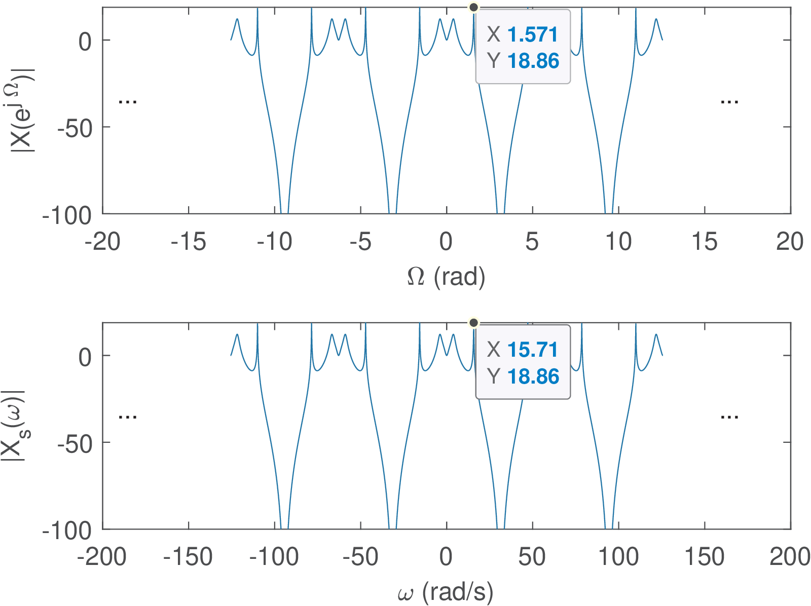
Figure 3.27: Result of converting $x [n]$ with spectrum $X (e^{j Ω})$ into $x_{s} (t)$ with $X_{s} (ω) = X (e^{jω T_{s}})$ via a DT/S conversion using $F_{s} = 10$ Hz.

The datatips in Figure 3.27 highlight that the value $| X (e^{j Ω_{0}}) | = 18.86$ at $Ω_{0} = 1.571$ rad was converted to $| X (ω_{0}) |$ where $ω_{0} = Ω_{0} F_{s} = 15.71$ rad/s.

The replicas that occur in the spectrum of a sampled signal are located in Nyquist zones, which are intervals of $F_{s} ∕ 2$ when the frequency $f$ is specified in Hertz. For example, the first Nyquist zone is $[0, F_{s} ∕ 2 [$ , the second is $[F_{s} ∕ 2, F_{s} [$ and so on. When the frequencies $ω$ and $Ω$ are specified in rad/s and rad, the bandwidths of the Nyquist zones are $π F_{s}$ and $π$ , respectively.

In summary, $X_{s} (ω)$ inherits the periodicity of $X (e^{j Ω})$ that corresponds to $X_{s} (ω + k 2 π F_{s}) = X_{s} (ω), k \in ℤ$ , but the notation does not indicate this periodicity. Therefore, in some situations, it is convenient to denote the spectrum of $x_{s} (t)$ as $X (e^{jω T_{s}})$ , which indicates that this spectrum is periodic as proven by

X_{s} (e^{j (ω + k 2 π F_{s}) T_{s}}) = X_{s} (e^{jω T_{s}} e^{jk 2 π}) = X_{s} (e^{jω T_{s}})

given that $e^{jk 2 π} = 1, \forall k$ .

Instead of using the angular frequency $ω$ in rad/s, an alternative description of a spectrum with period $F_{s} = 1 ∕ T_{s}$ is $X (e^{j 2 πf T_{s}})$ , using $f$ in Hz. This notation reminds that

X_{s} (e^{j 2 π (f + k F_{s}) T_{s}}) = X_{s} (e^{j 2 πf T_{s}} e^{j 2 πk}) = X_{s} (e^{j 2 πf T_{s}}),

which indicates this periodic spectrum has the same value at frequencies $f + k F_{s}$ that are multiples of $F_{s}$ .

Notation for combined filtering and DT/S stages

Assume a digital signal processing pipeline such as the one in Figure 1.42, in which a system function $H (z)$ (for instance, a digital filter) is implemented in the DSP block. The corresponding DTFT of $H (z)$ is $H (e^{j Ω})$ . The roles of these two stages:

x_{q} [n] \to H (z) \to y_{q} [n] \to DT/S \to y_{s} (t)

can be combined into one “analog” filter with frequency response $H (e^{jω T_{s}})$ . This can be interpreted as a simple abscissa scaling in graphs such as Figure 3.27. Another view is that, while Eq. (3.49) refers to a signal (a sampled signal in this case), the corresponding version of a DT/S process applied to a system (an analog system in this case) is

H (ω) = H (e^{j Ω}) |_{Ω = ω T_{s}} = H (e^{jω T_{s}}) .

(3.50)

In some cases, such as IIR filter design discussed in Section 3.7, it is useful to adopt subindices $z$ and $s$ to avoid confusion and disambiguate $H (z)$ and $H (s)$ within a signal processing pipeline. In this case, the previous equation is written as

H_{s} (ω) = H_{z} (e^{j Ω}) |_{Ω = ω T_{s}} = H_{z} (e^{jω T_{s}}),

(3.51)

which is similar to the simplified notation described in Example 3.24 for S/DT processes when using time-domain equations.

3.5 Improved Notation to Deal with DT/S and S/DT Conversions

3.5.1 Notation for signals and systems related to S/DT conversion

3.5.2 Notation for signals and systems related to DT/S conversion

Notation for combined filtering and DT/S stages