Linear Time-Invariant Systems and the Convolution

3.3 Linear Time-Invariant Systems and the Convolution

This section is dedicated to the study of linear and time-invariant (LTI) systems and the convolution operation.

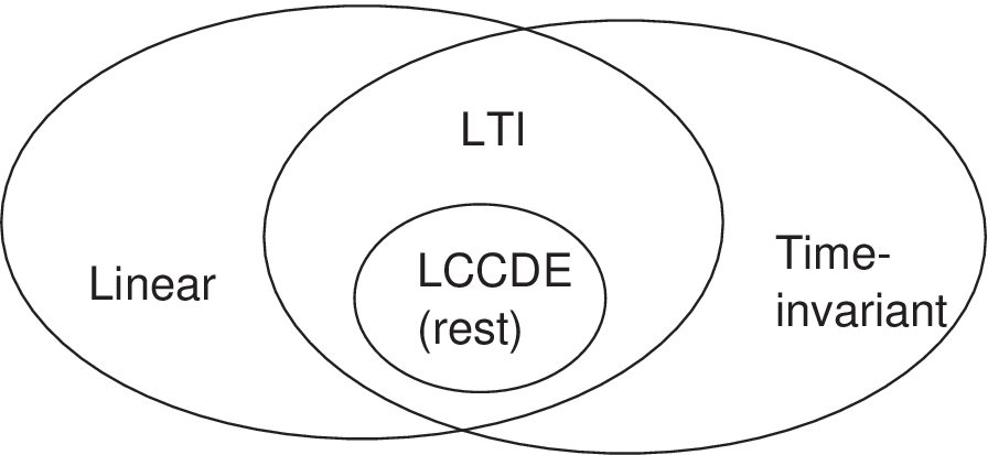
Figure 3.1: Diagram of systems, emphasizing the linear and time-invariant (LTI) systems and the systems described by linear, constant-coefficient differential (or difference) equations (LCCDE).

Figure 3.1 depicts the position of LTI systems and also includes the important subset of systems described by linear, constant-coefficient differential (or difference, in discrete-time) equations (LCCDE). In this text, it is assumed that the LCCDE systems have zero initial conditions or, equivalently, that the system is at rest.

3.3.1 Impulse response of a generic system

The impulse response of a system is the output signal when the input is an impulse. In continuous-time, the impulse response $h (t)$ corresponds to the output $y (t)$ when the input is $x (t) = δ (t)$ , which can be represented by:

δ (t) \to H \to h (t)

and in discrete-time this corresponds to:

δ [n] \to H \to h [n] .

An impulse response can be obtained for any system (e. g., a time-variant and non-linear system). But the impulse response is particularly important to LTI systems, as discussed in the next paragraphs.

3.3.2 Impulse response of LTI systems and the convolution operation

This subsection emphasizes discrete-time but the concepts are applied also to continuous-time signals and systems.

As mentioned in Section 3.2, a LTI system is completely characterized by its impulse response.¹ This means that, if $h [n]$ is known for a given LTI system, one can obtain the output $y [n]$ corresponding to a generic input $x [n]$ via the convolution operation, denoted as $y [n] = x [n] * h [h]$ . This was represented in Block (3.1), which is repeated below for convenience:

x [n] \to h [n] \to y [n] = x [n] * h [n] .

Example 3.1. Knowing the impulse response of a LTI system, it is possible to calculate the system’s output to any input. Assume that a system $H$ is LTI and its impulse response $h [n] = - 2 δ [n] + δ [n - 1] + 2 δ [n - 2]$ is obtained by imposing an input $x [n] = δ [n]$ and observing the output $y [n]$ . This special output is now denoted as $h [n]$ and it suffices to calculate new output signals $y [n]$ for any $x [n]$ .

For example, assuming $x [n] = 2 δ [n] - 3 δ [n - 1] + 4 δ [n - 2]$ , the corresponding system’s output is:

\begin{align} y [n] & = H {x [n]} \\ = H {2 δ [n] - 3 δ [n - 1] + 4 δ [n - 2]} \\ = H {2 δ [n]} + H {- 3 δ [n - 1]} + H {4 δ [n - 2]} & (using additivity) \\ = 2 H {δ [n]} - 3 H {δ [n - 1]} + 4 H {δ [n - 2]} & (using homogeneity) \\ = 2 h [n] - 3 h [n - 1] + 4 h [n - 2] & (using time-invariance) \\ = 2 (- 2 δ [n] + δ [n - 1] + 2 δ [n - 2]) - 3 (- 2 δ [n - 1] + δ [n - 2] + 2 δ [n - 3]) + \dots \\ 4 (- 2 δ [n - 2] + δ [n - 3] + 2 δ [n - 4]) \\ = - 4 δ [n] + 8 δ [n - 1] - 7 δ [n - 2] - 2 δ [n - 3] + 8 δ [n - 4] . & (3.2) \end{align}

This example illustrates the convolution, but it does not use the convolution equation explicitly. $□$

In general, the input/output relation of a LTI depends on the fact that any input $x [n]$ can be represented by impulses, and knowing the impulse response $h [n]$ (the output for a single impulse $δ [n]$ ) allows the output of the LTI system be obtained by invoking linearity and time-invariance, as done in Eq. (3.2). In summary:

As indicated by Eq. (1.4), any signal can be decomposed as the sum of impulses $αδ [n - n_{0}]$ that are shifted in time by $n_{0}$ and scaled in amplitude by $α$ .
By the time-invariance property of the system $H$ , each impulse $δ [n - n_{0}]$ applied to its input, generates a sequence $h [n - n_{0}]$ with the same delay $n_{0}$ at its output
and by the linearity property (more specifically, the homogeneity) of the system $H$ , if the input impulse $αδ [n - n_{0}]$ is scaled by $α$ , this constant shows up at the corresponding output parcel $αh [n - n_{0}]$ .
Finally, by the linearity property (more specifically, the additivity) of the system $H$ , the output parcels $αh [n - n_{0}]$ can be summed to composed $y [n]$ .

Generalizing the steps in Eq. (3.2), one obtains the convolution operation:

\begin{align} y [n] & = H {x [n]} = H {\sum_{k = - \infty}^{\infty} x [k] δ [n - k]} \\ = \sum_{k = - \infty}^{\infty} x [k] H {δ [n - k]} & (using linearity) \\ = \sum_{k = - \infty}^{\infty} x [k] h [n - k] (using time-invariance) & (3.3) \end{align}

Note that both linearity and time-invariance were invoked in this proof. The continuous-time convolution is similar:

y (t) = \int_{- \infty}^{\infty} x (τ) h (t - τ) dτ .

(3.4)

The convolution is so important that it is represented by the operator $*$ . For example, $y [n] = x [n] * h [n]$ denotes the convolution of $x [n]$ and $h [n]$ . Because $*$ is the same symbol used for multiplication in programming languages, the context has to distinguish them.

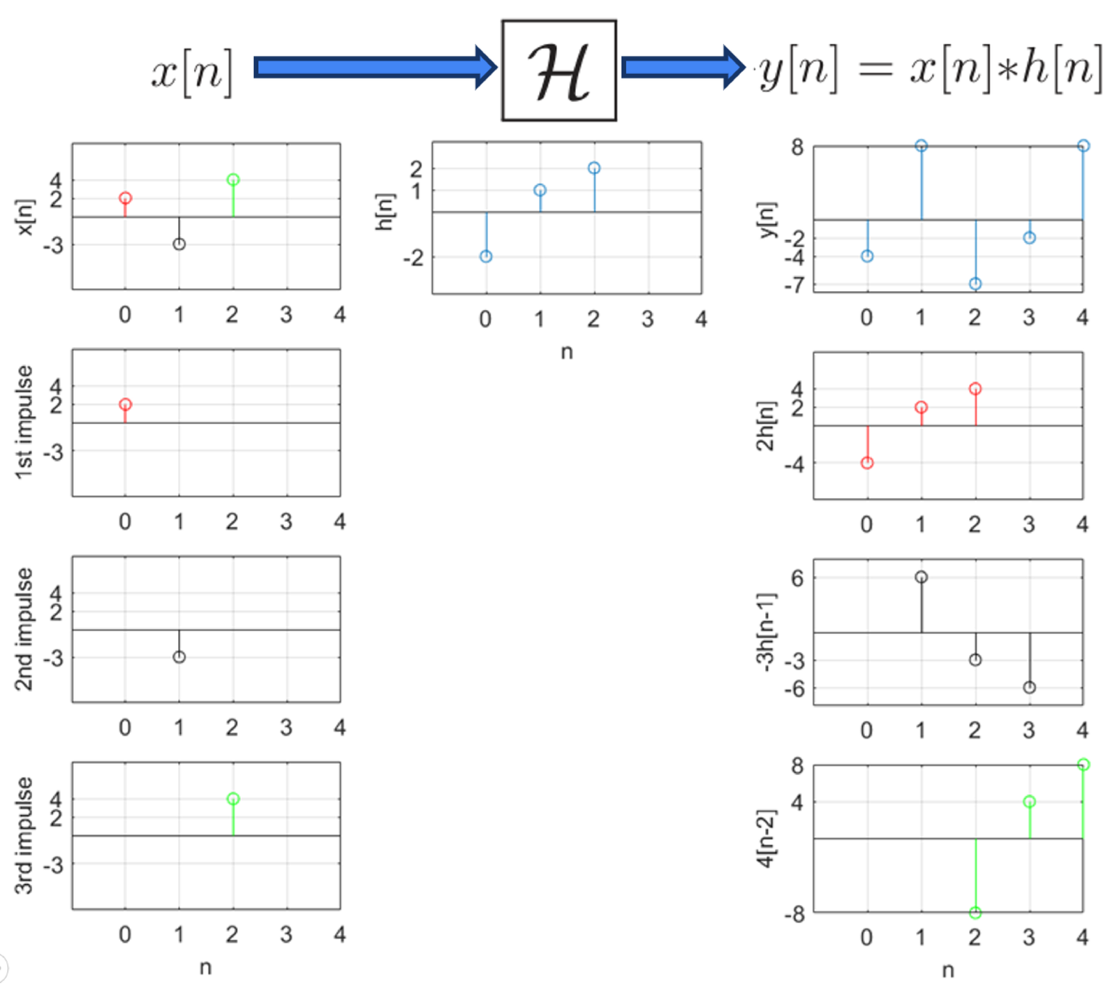
Figure 3.2: Example of convolution between $x [n] = 2 δ [n] - 3 δ [n - 1] + 4 δ [n - 2]$ and $h [n] = - 2 δ [n] + δ [n - 1] + 2 δ [n - 2]$ . The top-left and top-right plots are $x [n]$ and $y [n]$ , respectively, and surround $h [n]$ graph. The other plots are the three impulses of $x [n]$ (left) and the corresponding parcels that compose $y [n]$ (right).

Figure 3.2 illustrates the convolution discussed in Example 3.1. The interpretation is that $y [n]$ is composed by the sum of several scaled and shifted impulse responses. In this case, because $x [n]$ is composed of three impulses, the output $y [n]$ can be obtained by adding up the three versions of $h [n]$ created by each impulse. The three plots at the bottom-right in Figure 3.2 indicate that $y [n]$ is the sum of $2 h [n]$ , $- 3 h [n - 1]$ and $4 h [n - 2]$ , due to the input impulses $2 δ [n]$ , $- 3 δ [n - 1]$ and $4 δ [n - 2]$ , respectively.

If the impulse response completely characterizes a LTI system, all its properties can be inferred from the corresponding impulse response. This is discussed in Appendix B.7.7.

3.3.3 Convolution properties

For both continuous-time and discrete-time, the convolution has the following properties:

Commutative: $a * b = b * a$
Associative: $a * (b * c) = (a * b) * c$
Distributive: $a * (b + c) = a * b + a * c$

The commutative property of the convolution, allows to rewrite it using two equivalent expressions:

y [n] = \sum_{k = - \infty}^{\infty} x [k] h [n - k] = ∑_{k = - \infty}^{\infty} h [k] x [n - k] .

(3.5)

The next two block diagrams represent the same concept of Eq. (3.5) because

x [n] \to h [n] \to y [n] = x [n] * h [n] .

and

h [n] \to x [n] \to y [n] = h [n] * x [n] .

lead to the same output $y [n]$ .

Two other facts about the discrete-time convolution, which have similar continuous-time counterparts:

Duration of a convolution output. If $N_{1}$ and $N_{2}$ are the duration in samples of two finite-length discrete-time sequences $a [n]$ and $b [n]$ , then $a [n] * b [n]$ has duration $N_{1} + N_{2} - 1$ samples.
Relation among indices of signals involved in a convolution. Given the convolution equation $y [n] = \sum_{k = - \infty}^{\infty} x [k] h [n - k]$ , considering a specific index $n$ of the output, one can note that all parcels in the summation are obtained by multiplying $x [k]$ and $h [n - k]$ such that the summation of this pair of indices $(k, n - k)$ is always $n$ . In other words, if $a [n] = b [n] * c [n]$ , to obtain $a [n_{a}]$ for a specific instant $n_{a}$ , one sums all valid products $b [n_{b}] c [n_{c}]$ such that $n_{a} = n_{b} + n_{c}$ .

Example 3.2. Example regarding the relation among indices of signals involved in a convolution. To verify the previously mentioned fact, consider the convolution between $x 1 [n] = δ [n] + 2 δ [n - 1] + 3 δ [n - 2]$ and $x 2 [n] = 5 δ [n] + 6 δ [n - 1] + 7 δ [n - 2] + 8 δ [n - 3]$ . The output $y [n] = x 1 [n] * x 2 [n]$ is given by

y[0] = x1[0] x2[0] = 5
y[1] = x1[0] x2[1] + x1[1] x2[0] = 16
y[2] = x1[0] x2[2] + x1[1] x2[1] + x1[2] x2[0] = 34
y[3] = x1[0] x2[3] + x1[1] x2[2] + x1[2] x2[1] = 40
y[4] = x1[1] x2[3] + x1[2] x2[2] = 37
y[5] = x1[2] x2[3] = 24

where one can note that the indexes of the input sequences sum up to the index of the output. For instance, considering $n_{a} = 2$ , the value $y [n_{a}] = y [2]$ is obtained by adding three parcels $x 1 [n_{b}] x 2 [n_{c}]$ in which $n_{a} = n_{b} + n_{c} = 2$ : $(n_{b} = 0, n_{c} = 2)$ , $(n_{b} = 1, n_{c} = 1)$ and $(n_{b} = 2, n_{c} = 0)$ . $□$

Example 3.3. Example regarding the duration of a convolution output. The finite-duration sequences of Example 3.2 also help to illustrate the duration of a convolution output. The sequence $x 1 [n]$ starts at $n = 0$ and ends at $n = 2$ , which accounts for a duration (also called support) of $N_{1} = 3$ samples. Sequence $x 2 [n]$ starts at $n = 0$ and ends at $n = 3$ , which accounts for a support of $N_{2} = 4$ samples. Hence, the output $y [n]$ has a duration of $N_{1} + N_{2} - 1 = 3 + 4 - 1 = 6$ samples, starting from $n = 0$ and ending at $n = 5$ .

It should be noticed that the duration of a sequence that has some zeroed amplitudes located between non-zero samples should consider the “internal” zeroed samples when determining the sequence support. For instance, the duration of $x_{1} [n] = δ [n] + 2 δ [n - 4]$ is $N_{1} = 5$ samples. $□$

3.3.4 Fourier convolution property

The convolution property of Fourier transforms states that the convolution between two signals has a Fourier transform given by the multiplication of their Fourier transforms. In other words, the convolution between these signals by can be obtained as the inverse Fourier transform of the multiplication of their Fourier transforms. For example, assuming continuous-time, the convolution $y (t) = x_{1} (t) * x_{2} (t)$ can be obtained with

y (t) = F^{- 1} {X_{1} (f) X_{2} (f)},

(3.6)

where $X_{1} (f)$ and $X_{2} (f)$ are the corresponding Fourier transforms. Similarly, in discrete-time, the convolution result $y [n]$ can be written as

y [n] = x_{1} [n] * x_{2} [n] = {DTFT}^{- 1} {X_{1} (e^{j Ω}) X_{2} (e^{j Ω})},

(3.7)

where $X_{1} (e^{j Ω})$ and $X_{2} (e^{j Ω})$ are the corresponding DTFTs and, in this case, $F^{- 1}$ denotes the inverse DTFT.

Example 3.4. Convolution using DTFTs and inverse DTFT. For example, if $x_{1} [n] = α_{1}^{n} u [n]$ and $x_{2} [n] = α_{2}^{n} u [n]$ are two discrete-time complex exponentials with $| α_{1} | < 1$ and $| α_{2} | < 1$ , their DTFTs are $X_{i} (e^{j Ω}) = 1 ∕ (1 - α_{i} e^{- j Ω}), i = 1, 2$ , respectively. The convolution result is

y [n] = x_{1} [n] * x_{2} [n] = \frac{1}{α_{1} - α_{2}} (α_{1}^{n + 1} u [n] - α_{2}^{n + 1} u [n])

(3.8)

and can be obtained via the inverse DTFT of $Y (e^{j Ω})$ , which is given by

Y (e^{j Ω}) = X_{1} (e^{j Ω}) X_{2} (e^{j Ω}) = \frac{1}{(1 - α_{1} e^{- j Ω}) (1 - α_{2} e^{- j Ω})} .

(3.9)

Eq. (3.8) can be obtained by using partial fraction expansion of Eq. (3.9). $□$

3.3.5 Fourier multiplication property

Due to the duality of Fourier transforms, the multiplication in time-domain corresponds to convolution in frequency-domain between the respective spectra. This is called the multiplication property and corresponds to

x_{1} (t) x_{2} (t) \Leftrightarrow X_{1} (f) * X_{2} (f) = \int_{- \infty}^{\infty} X_{1} (p) X_{2} (f - p) d p .

(3.10)

in continuous-time.

In discrete-time, one needs to take in account that the spectra are periodic and the conventional convolution is not adequate when both signals are periodic. In fact, the multiplication property for discrete-time signals is

x_{1} [n] x_{2} [n] \Leftrightarrow \frac{1}{2 π} \int_{< 2 π >} X (e^{j Ω}) X_{2} (e^{j (Ω - 𝜃)}) d𝜃 .

(3.11)

The integral in Eq. (3.11) differs from a conventional convolution because it is calculated over only one period ( $2 π$ rad in this case) and the result is normalized by this period. This modified convolution is denoted as $⊛$ and is called periodic, cyclic or circular convolution. As in a Fourier series expansion to obtain coefficients $c_{k}$ , the associated period must be known in order to properly use $⊛$ . The normalization by the period can be incorporated in its definition, which leads to the following expression for the periodic convolution:

x_{1} (t) ⊛ x_{2} (t) = \frac{1}{T} \int_{< T >} x_{1} (τ) x_{2} (t - τ) d τ,

(3.12)

where both signals are periodic in $T$ .

The definition of Eq. (3.12) allows to write Eq. (3.11) as

x_{1} [n] x_{2} [n] \Leftrightarrow X (e^{j Ω}) ⊛ X_{2} (e^{j Ω}),

(3.13)

where the period $2 π$ is implicit.

The periodic convolution corresponds to performing the conventional convolution (called “linear” convolution, in contrast to “circular”) between $x_{1} (t)$ and $x'_{2} (t)$ , where $x'_{2} (t)$ is a single period of $x_{2} (t)$ that is normalized by the period $T$ . The interval to define $x'_{2} (t)$ can be conveniently chosen as $x_{2}^{'} (t) = x_{2} (t) ∕ T, 0 \leq t < T$ , or $0$ otherwise, or $x_{2}^{'} (t) = x_{2} (t) ∕ T, - T ∕ 2 \leq t < T ∕ 2$ , or $0$ otherwise.

As discussed in the sequel, the periodic convolution is typically associated to FFT-based processing.

3.3.6 Distinct implementations of convolution

The next subsections will discuss some alternative implementations of convolution between two discrete-time signals $x [n]$ and $h [n]$ . For simplicity, both signals are assumed to start at $n = 0$ , having zero amplitude for $n < 0$ . When using a programming language (Python, Matlab/Octave, etc.), it is often necessary to explicitly deal with and generate the time indexes. More generally, an implementation of convolution that supports the signals to start at arbitrary time instants requires the corresponding information about the abscissas of $x [n]$ and $h [n]$ . In contrast, the convolution routines described in the next subsections require only two vectors as input arguments, corresponding to the amplitudes of $x [n]$ and $h [n]$ .

Implementation based on linearity and time-invariance

Listing 3.1 provides a straight and pedagogical implementation of convolution between two discrete-time sequences.² This implementation mimics the processing in Figure 3.2, where the three parcels $x [k] h [n - k]$ are added to compose $y [n]$ .

Listing 3.1: PythonFunctions/ak_convolution.py

1import numpy as np 
2 
3 
4def ak_convolution(x: np.ndarray, h: np.ndarray) -> np.ndarray: 
5    """Convolution between sequences x and h using LIT properties.""" 
6    Nx = len(x)              # number of samples in x 
7    Nh = len(h)              # number of samples in h 
8    N = Nx + Nh - 1          # number of samples in output y 
9    y = np.zeros(N)          # pre-allocate space for y[n] 
10    for k in range(Nx): 
11        # create indices n = k, k+1, ..., k+Nh-1 to mimic h[n-k] 
12        n_range_with_delay_k = np.arange(k, k + Nh) 
13        # add contribution of x[k] * h[n-k] to y[n] 
14        y[n_range_with_delay_k] += x[k] * h  # y[n] += x[k] h[n-k] 
15    return y 
16 
17 
18if __name__ == "__main__":  # Example usage 
19    x = np.array([2, -3, 4]) 
20    h = np.array([-2, 1, 2]) 
21    y = ak_convolution(x, h) 
22    print("x =", x), print("h =", h), print("y =", y)

As expected, the output of Listing 3.1 is y = [-4. 8. -7. -2. 8.]. One thing to notice about Listing 3.1 is that it requires accumulating several parcels until getting the final output value $y [n_{0}]$ for a given time instant $n_{0}$ . For instance, the value $y [2] = - 7$ is obtained only after adding the contributions $4 + (- 3) + (- 8)$ from all three parcels of Example 3.1 (and Figure 3.2). This implementation is very pedagogical with respect to using the properties of a LTI system but has practical inconveniences. For instance, as indicated in Listing 3.1, this implementation requires pre-allocating space for output $y [n]$ . The next subsection discusses an alternative implementation that is more appropriate to practical signal processing.

Implementation based on convolution equation and its graphical interpretation

The next paragraphs discuss the convolution implementation of Listing 3.2. In this implementation, for each time instant $n$ , the value of the output $y [n]$ is calculated considering all corresponding parcels and accumulated in a variable called acc.

Listing 3.2: PythonFunctions/ak_causalconvolution.py

1def ak_causal_convolution2(x: np.ndarray, h: np.ndarray) -> np.ndarray: 
2    """ Convolution assuming causal finite-length sequences.""" 
3    Nx = len(x)              # number of samples in x 
4    Nh = len(h)              # number of samples in h 
5    N = Nx + Nh - 1          # number of samples in output y 
6    y = list()        # initialize an empty list to store the convolution 
7    for n in range(N): 
8        # find the valid range of k for each value of n 
9        kmin = max(0, n - (Nh - 1)) 
10        kmax = min(Nx - 1, n) 
11        acc = 0  # accumulator variable for calculating y[n] 
12        for k in range(kmin, kmax + 1): 
13            acc += x[k] * h[n - k] 
14        y.append(acc)  # append the calculated value of y[n] to the list y 
15    return np.array(y)

In Listing 3.2, the values of $y [n]$ are computed and stored in a list. But in an embedded system implementing DSP, this value of $y [n]$ could be written to a DAC chip, for instance, and not stored. The range of valid $k$ values is determined by considering that $x [n]$ exists only for $0 \leq n \leq N_{x} - 1$ , while $h [n]$ exists only for $0 \leq n \leq N_{h} - 1$ , For a term $x [k] h [n - k]$ to contribute to the convolution, both samples must exist simultaneously. In more details, considering the duration of $x [k]$ , one has:

k \geq 0 and k \leq N_{x} - 1 .

Now, for a given value of $n$ , the duration of $h [n - k]$ leads to $n - k \geq 0$ and $n - k \leq N_{h} - 1$ , which can be written as

k \geq n - (N_{h} - 1) and k \leq n .

Combining the requirements leads to the range indicated in Listing 3.2 for kmin and kmax.

Based on the commutative property of the convolution in Eq. (3.5), the roles of $x [n]$ and $h [n]$ can be swapped, and an equivalent implementation of the loop in Listing 3.2 can be found in Listing 3.3.

Listing 3.3: PythonFunctions/ak_causalconvolution2.py

1    for n in range(N): 
2        # find the valid range of k for each value of n 
3        kmin = max(0, n - (Nx - 1)) 
4        kmax = min(Nh - 1, n) 
5        acc = 0  # accumulator variable for calculating y[n] 
6        for k in range(kmin, kmax + 1): 
7            acc += h[k] * x[n - k] 
8        y.append(acc)  # append the calculated value of y[n] to the list y

The implementation in Listing 3.3 has a convenient graphical interpretation. To calculate the convolution output $y [n] = x [n] * h [n]$ for a given value of $n = n_{0}$ , the loop over the operation acc += h[k] * x[n - k] corresponds to:

f 1.: The index $n$ is a fixed integer $n_{0}$ and the complete sequences $x [n]$ and $h [n]$ are indexed via an auxiliary integer number $k$ .
f 2.: one or both sequences $x [n]$ and $h [n]$ may have finite duration, but the range of $k$ is assumed to be $] - \infty, \infty [$ for generality.
f 3.: the value of $y [n_{0}]$ is obtained by multiplying the sequences $h [k]$ and $x [n_{0} - k]$ , and summing the non-zero parcels.
f 4.: the sequence $x [n_{0} - k]$ is obtained by flipping $x [k]$ over the y-axis and shifting by $n_{0}$ (to the right if $n_{0} > 0$ or to the left in case $n_{0} < 0$ ).
f 5.: for a new value of $n$ , say $n = n_{1} = n_{0} + 1$ , the sequence $x [n_{1} - k]$ is obtained and the process is repeated.

A similar procedure can be adopted for continuous-time signals, with the summations in discrete-time being substituted by integrals.

Example 3.5. Example of graphical interpretation of convolution.

The convolution example in Figure 3.2 was based on interpreting the properties of a LTI system. But, as discussed, the procedure based in Listing 3.3 is more appropriate in some occasions, such as when implementing convolution in real-time systems. Hence, Figure 3.3 provides an alternative view for obtaining the convolution in Figure 3.2.

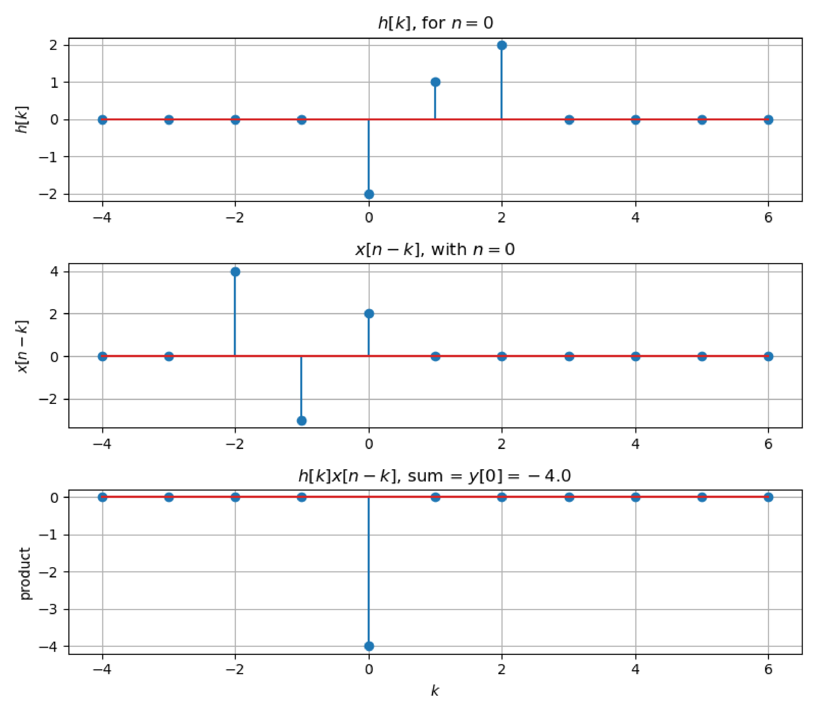
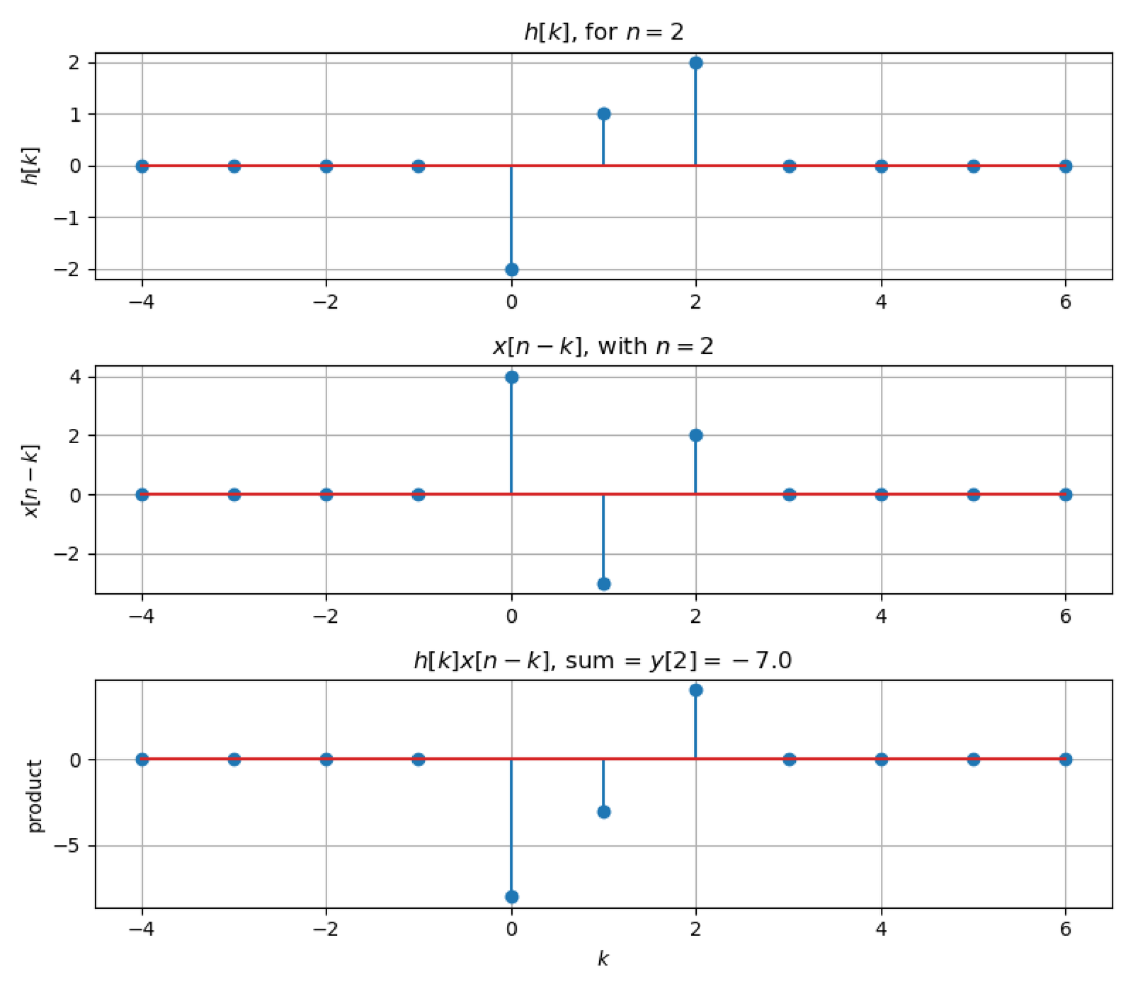
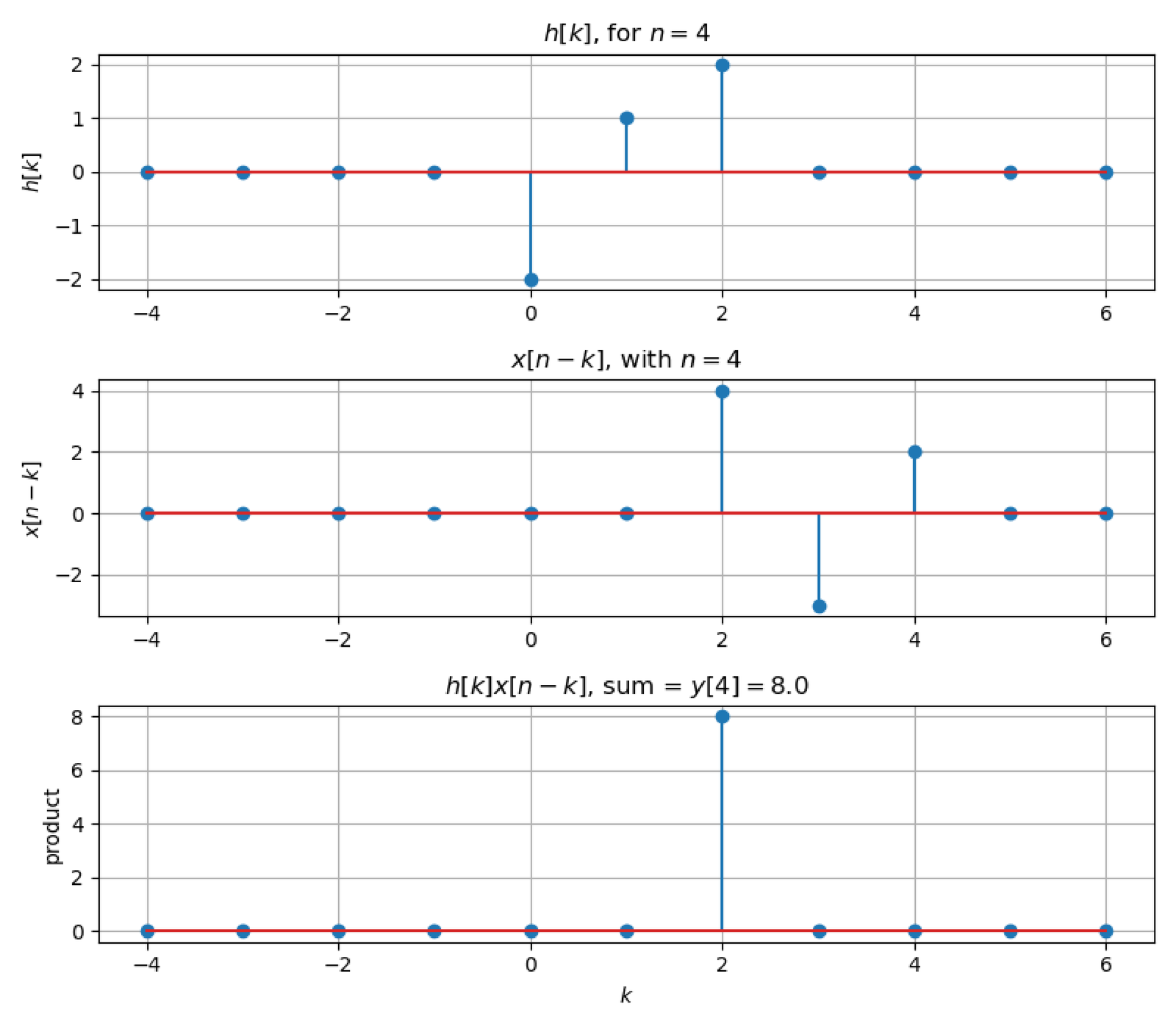
To obtain the output sample $y [0]$ , Figure 3.2a shows the sequences $h [k]$ and $x [n - k]$ when $n = 0$ . In this case, the only non-zero parcel in the product is the value $- 4$ in $k = 0$ . Similarly, Figure 3.2c shows that the sequences multiplication have a single non-zero parcel when $n = 4$ . In contrast, Figure 3.2b shows that $y [2]$ is obtained by the summation of three non-zero parcels, at $k = 0, 1$ and $2$ . $□$

Implementation based on polynomial multiplication

If the samples of two finite-length sequences $x [n]$ and $h [n]$ are organized as coefficients of two polynomials, linear convolution becomes equivalent to polynomial multiplication. For the example in Figure 3.2 one can obtain the convolution result by multiplying the equivalent polynomials $2 u^{2} - 3 u + 4$ and $- 2 u^{2} + u + 2$ , which leads to $- 4 u^{4} + 8 u^{3} - 7 u^{2} - 2 u + 8$ , i. e., the coefficients are the samples of $y [n]$ .

Implementation of circular and linear convolutions using FFT

Recalling that the FFT corresponds to sampling the DTFT, Eq. (3.7) suggests that FFTs can be used to efficiently compute a convolution. However, even if $x [n]$ were not periodic, when its DTFT $X (e^{j Ω})$ is sampled (in frequency domain) by the FFT, the FFT values $X [k]$ are representing the spectrum of a periodic version of $x [n]$ . Consequently, when FFTs substitute DTFTs in Eq. (3.7), the result is not the linear but the circular convolution represented as

y [n] = x_{1} [n] ⊛ x_{2} [n] = {FFT}^{- 1} {X_{1} [k] X_{2} [k]},

(3.14)

where both FFTs must have the same length $N$ , which plays the whole of the period of a circular convolution.

Listing 3.4 provides an example of using Eq. (3.14). Note how zero-padding is used to assure the element-wise multiplication fft(x,N).*fft(h,N) uses arrays with the same length. The result of Listing 3.4 confirms that, in general, linear and circular convolution differ.

Listing 3.4: MatlabOctaveCodeSnippets/snip_systems_circularConvolution.m. [ Python version]

1x=[1 2 3 4]; h=[.9 .8]; %signals to be convolved 
2shouldMakeEquivalent=0 %in general, linear and circular conv. differ 
3if shouldMakeEquivalent==1 
4    N=length(x)+length(h)-1; %to force linear and circular coincide 
5else 
6    N=max(length(x),length(h)); %required for FFT zero-padding 
7end 
8linearConv=conv(x,h) %linear convolution 
9circularConv=ifft(fft(x,N).*fft(h,N)) %circular convolution, N=4 
10%circularConv=cconv(x,h,N) %note that Matlab has the cconv function

If the value of shouldMakeEquivalent is made equal to 1, Listing 3.4 returns the same results for both linear and circular convolutions. In fact, when the FFT length is at least the number of non-zero samples of the convolution output, the circular and linear convolution results coincide. This suggests that Eq. (3.14) can be used to calculate a linear convolution, provided that the FFT length is made long enough.

When small vectors are involved, a direct convolution implementation using Listing 3.1 or Listing 3.2 is efficient. But for large vectors, most DSP libraries adopt a FFT-based implementation because it is faster than direct convolution.

Implementation of convolution using FFT with infinite-duration signals

Obtaining a linear convolution via FFTs is trickier when one of the signals to be convolved has infinite duration. In this case, it is obviously not possible to find a large enough FFT length to use Eq. (3.14). However, if the other signal has finite duration, it is feasible and often used in practice to segment the long signal into blocks and calculate the linear convolution by sequentially calculating one FFT per block and properly combining the results. There are basically two alternatives to combine the intermediate results that are called overlap-add and overlap-save methods, and are roughly equivalent. Listing 3.5 illustrates the former.

Listing 3.5: MatlabOctaveCodeSnippets/snip_systems_overlapAdd.m. [ Python version]

1x=1:1000; %infinite duration (or "long") input signal 
2h=ones(1,3); %non-zero samples of finite-length impulse response 
3Nh=length(h); %number of impulse response non-zero samples 
4Nb=5; %block (segment) length 
5Nfft=2^nextpow2(Nh+Nb-1); %choose a power of 2 FFT size 
6Nx = length(x); %number of input samples 
7H = fft(h,Nfft); %pre-compute impulse response DFT, with zero-padding 
8beginIndex = 1; %initialize index for first sample of current block 
9y = zeros(1,Nh+Nx-1); %pre-allocate space for convolution output 
10while beginIndex <= Nx %loop over all blocks 
11    endSample = min(beginIndex+Nb-1,Nx);%last sample of current block 
12    Xblock = fft(x(beginIndex:endSample),Nfft); %DFT of block 
13    yblock = ifft(Xblock.*H,Nfft); %get circular convolution result 
14    outputIndex  = min(beginIndex+Nfft-1,Nh+Nx-1); %auxiliary variab. 
15    y(beginIndex:outputIndex) = y(beginIndex:outputIndex) + ... 
16        yblock(1:outputIndex-beginIndex+1); %add parcial result 
17    beginIndex = beginIndex+Nb; %shift begin of block 
18end 
19stem(y-conv(x,h)) %compare the error with result from conv

A typical application of the overlap-add and overlap-save methods is to compute the output of a LTI system represented by a finite-duration impulse response (i. e., a FIR filter, as will be discussed in Section 3.10). Listing 3.5 provides an example where the impulse response has only three non-zero samples, and the long input signal is segmented in blocks of Nb=5 samples.

Advanced: Convolution via correlation and vice-versa

Given that convolution and cross-correlation are tightly related, Listing 3.6 illustrates how the Matlab/Octave correlation function xcorr can be used to calculate convolution (conv) and vice-versa.

Listing 3.6: MatlabOctaveCodeSnippets/snip_systems_convolution_correlation.m. [ Python version]

1x=(1:4)+j*(4:-1:1); %define some complex signals as row vectors, such 
2y=rand(1,15)+j*rand(1,15); %that fliplr inverts the ordering 
3%% Correlation via convolution 
4Rref=xcorr(x,y); %reference of a cross-correlation 
5xcorrViaConv=conv(x,conj(fliplr(y))); %use the second argument 
6%% Convolution via correlation 
7Cref=conv(x,y); %reference of a convolution 
8convViaXcorr=xcorr(x,conj(fliplr(y))); %using the second argument 
9%convViaXcorr=conj(fliplr(xcorr(conj(fliplr(x)),y))); %alternative 
10%% Make sure they have the same length and compare the results 
11if length(x) ~= length(y) %this case requires post-processing because 
12    %xcorr assumes the sequences have the same length and uses 
13    %zero-padding if they do not. We treat the effect of these zeros: 
14    convolutionLength=length(x)+length(y)-1; 
15    correlationLength=2*max(length(x),length(y))-1; 
16    if length(x) < length(y) %zeros at the end 
17        convViaXcorr = convViaXcorr(1:convolutionLength); 
18        xcorrViaConv = [xcorrViaConv zeros(1,correlationLength- ... 
19            length(xcorrViaConv))]; 
20    elseif length(x) > length(y) %zeros at the beginning 
21        convViaXcorr = convViaXcorr(end-convolutionLength+1:end); 
22        xcorrViaConv = [zeros(1,correlationLength- ... 
23            length(xcorrViaConv)) xcorrViaConv]; 
24    end 
25end 
26ErroXcorr= max(abs(Rref - xcorrViaConv)) %calculate maximum errors 
27ErroConv = max(abs(Cref - convViaXcorr)) %should be small numbers

As indicated in Listing 3.6, the key step to mimic a convolution via correlation or vice-versa is to flip the signal using $x (- t)$ , use its complex conjugate and eventually shift by $t_{0}$ as indicated in

\hat{x} (t) = x^{*} (- t + t_{0}) .

(3.15)

Advanced: Discrete-time convolution in matrix notation

Convolution can be denoted in matrix notation. This is especially convenient when dealing with finite-duration discrete-time signals. When these signals are represented by column vectors $x_{1}$ and $x_{2}$ , a convolution matrix $H_{1}$ allows to obtain the convolution result $y = x_{1} * x_{2}$ as

y = H_{1} x_{2},

(3.16)

where $H_{1}$ is composed by the elements of $x_{1}$ . Because convolution is commutative, it is also possible to create $H_{2}$ from the elements of $x_{2}$ and use $y = H_{2} x_{1}$ .

This can be better understood with examples. Considering the goal is to obtain the convolution of two column vectors x1=[1; 2; 3] and x2=[5; 6; 7; 8] (previous example), instead of using y=conv(x1,x2), one can create a matrix

hmatrix = [
     1     0     0     0
     2     1     0     0
     3     2     1     0
     0     3     2     1
     0     0     3     2
     0     0     0     3]

with the command hmatrix = convmtx(x1,length(x2)), and then calculate the convolution with y=hmatrix * x2. Note that when using row vectors, the commands could be hm = convmtx(x1,length(x2)); x2*hm (in this case, hm would be the transpose of hmatrix). Application 3.4 discusses the issue of repeatedly processing blocks of samples using the convolution in matrix notation. The matrices created by convmtx are Toeplitz matrices and the command toeplitz.m can also be useful to compose convolution matrices.

3.3.7 Approximating continuous-time via discrete-time convolution

Some situations require approximating the continuous-time convolution denoted by Eq. (3.4) via the discrete-time convolution in Eq. (3.3). In such cases, the sampling interval $T_{s}$ should be used as a normalization factor, as indicated in Eq. (A.28). This factor is adopted in the next example.

Example 3.6. Convolution of a pulse with itself leads to a triangular waveform. Assume a pulse $p (t) = 4 rect (5 t - 0.1)$ (see $rect (\cdot)$ in Section 1.3.6) with amplitude $A = 4$ V and support $T_{0} = 0.2$ s. The convolution $p (t) * p (t)$ corresponds to a triangular waveform: it is 0 for $t < 0$ and assumes its maximum value at $A^{2} T_{0} = 4^{2} \times 0.2 = 3.2$ at 0.2 s, which corresponds to the time that the two pulses overlap completely and $A^{2} T_{0}$ is the area of $p^{2} (t)$ . Figure 3.4 depicts both the pulse and continuous-time convolution $p (t) * p (t)$ .

Figure 3.4: Convolution of a pulse $p (t) = 4 rect (5 t - 0.1)$ with itself, obtained with Listing 3.7.

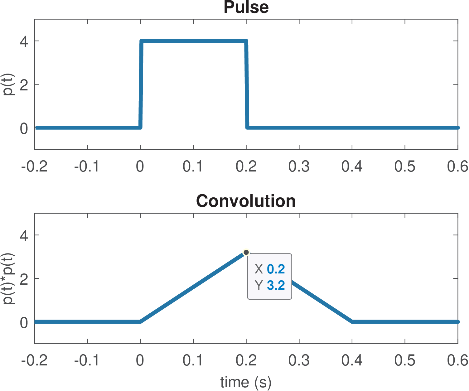
But Figure 3.4 was in fact obtained by representing $p (t)$ via its discrete-time version $p [n]$ , and approximating the convolution $p (t) * p (t)$ with the scaled discrete-time convolution $T_{s} (p [n] * p [n])$ , i. e., Eq. (A.28). Listing 3.7 shows the first lines of the script that generated Figure 3.4. After running Listing 3.7, the vectors pulse and triangle are shown in Figure 3.4 with the proper time axes.

Listing 3.7: MatlabOctaveCodeSnippets/snip_systems_continuous_discrete_conv

1T0=0.2; %pulse "duty cycle" (interval with non-zero amplitude): 0.2 s 
2Ts=2e-3; %sampling interval: 2 ms 
3N=T0/Ts; %number of samples to represent the pulse "duty cycle" 
4A=4; %pulse amplitude: 4 Volts 
5pulse=A*[zeros(1,N) ones(1,N) zeros(1,4*N)]; %pulse 
6triangle=Ts*conv(pulse,pulse); %(approximated) continuous convolution 
7disp(['Convolution peak at ' num2str(T0) ' is ' num2str(A^2*T0)])

Note in line 6 the scaling factor $T_{s}$ , which leads to the correct values, as indicated by the datatip in Figure 3.4. $□$

¹ Say you meet a person who tells you that he or she is an LTI system. You should then ask for his or her impulse response. If you know it, just relax, because you can perfectly calculate the person’s reaction (output) to any situation (input).

² On the Web one can find applets instructing about continuous and discrete convolution (see, e. g., [ url3cde]).