B.3  Probability Concepts for Signal Processing

This appendix provides a brief overview of probability concepts relevant to digital signal processing.

B.3.1  Joint and Conditional Probability

Let $A$ and $B$ be two events. Their joint probability, denoted by $P(A,B)$ (or equivalently $P(A\cap B)$), quantifies the probability that both events occur.

The conditional probability of $B$ given $A$ is defined as

Equivalently, the joint probability can be written as

Two events $A$ and $B$ are said to be independent if

which implies that

Example B.1. Fair coin. Consider two independent tosses of a fair coin. Let $A$ be the event “the first toss results in heads” and $B$ the event “the second toss results in heads.” Then $P(A)=P(B)=0.5$, and

Moreover, $P(B\mid A)=P(B)$, reflecting the independence of the two events.   $\text{□}$

Starting from the two equivalent factorizations of the joint probability,

we obtain

which is known as Bayes’ rule (see, e. g., [ urlBMpro]).

Although the notation $P(B\mid A)$ may suggest that $A$ influences $B$, conditional probability does not, in general, imply a causal relationship.

B.3.2  Random variables

Understanding the application of probability concepts into signal processing requires distinguishing three concepts: experiment outcomes, events, and random variables. A random variable maps outcomes into numbers as detailed below.

The outcome of a probabilistic experiment is not necessarily a number, but an element $\omega$ of a set $\mathrm{\Omega }$, called the sample space. For example, when tossing a coin, the outcome can be $\omega =\text{heads}$ or $\omega =\text{tails}$.

A random variable provides a way to assign numerical values to these outcomes. Formally, a random variable $X$ is a function

which associates a real number $X(\omega )$ with each outcome $\omega \in \mathrm{\Omega }$. (More generally, random variables may take values in $ℂ$, vectors, etc., but here we restrict attention to real-valued variables.)

A common source of confusion is the notation. In standard mathematical notation, a function is written as $y=f(x)$, where $f$ is the function and $y$ is its output. In probability, however, it is customary to use the same symbol $X$ both for the function (the random variable) and for its values. Strictly speaking, the numerical value is $X(\omega )$, but in practice we often write simply $X$. This is an abuse of notation that must be understood from context.

Every random variable induces a probability distribution on the real line. If the set of possible values of $X$ is finite or countable, $X$ is called a discrete random variable and is described by a probability mass function. If $X$ takes values in a continuum, it is called a continuous random variable and is described (when it exists) by a probability density function.

In summary, a random variable is a function and its “randomness” comes from the randomness of its input $\omega$, not from the function itself.

First note that the outcome of a probabilistic experiment need not be a number but any element of a set $\mathrm{\Omega }$ of possible outcomes. For example, the outcome when a coin is tossed can be $\omega =$“heads” or $\omega =$“tails”. Basically, random variables allow us to map any probabilistic event into numbers, which are then conveniently manipulated using mathematical operations such as integral and derivatives. A source of confusion is that, strictly, a random variable (e.g., $X$ or $Y$) is a function. More specifically, a random variable (r.v.) is a function $X:\mathrm{\Omega }\to ℝ$ that associates a unique numerical value with every outcome of an experiment (r.v. can be complex numbers, vectors, etc., but here it will be assumed as a real number). In math, a function output is often represented as $y=f(x)$. When dealing with a r.v., instead of adopting something like $X(\omega )$, both the random variable (equivalent to the function $f$) and its output value (equivalent to $y$) is represented by a single letter (e.g., $X$ or $Y$).

There are two types of r.v.: discrete and continuous. Hence, a r.v. has either an associated probability distribution (discrete r.v.) or probability density function (continuous r.v.).

Assume a discrete r.v. $X$ and a continuous r.v. $Y$. While the former is typically described by a probability mass function (pmf), the latter can be described by a probability density function (pdf).

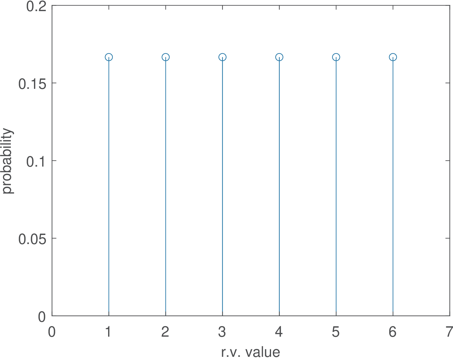
Say that $X$ represents the outcome of rolling a dice. Its PMF is shown in Figure B.1 and indicates that each face of a fair dice has a probability of $1∕6$.

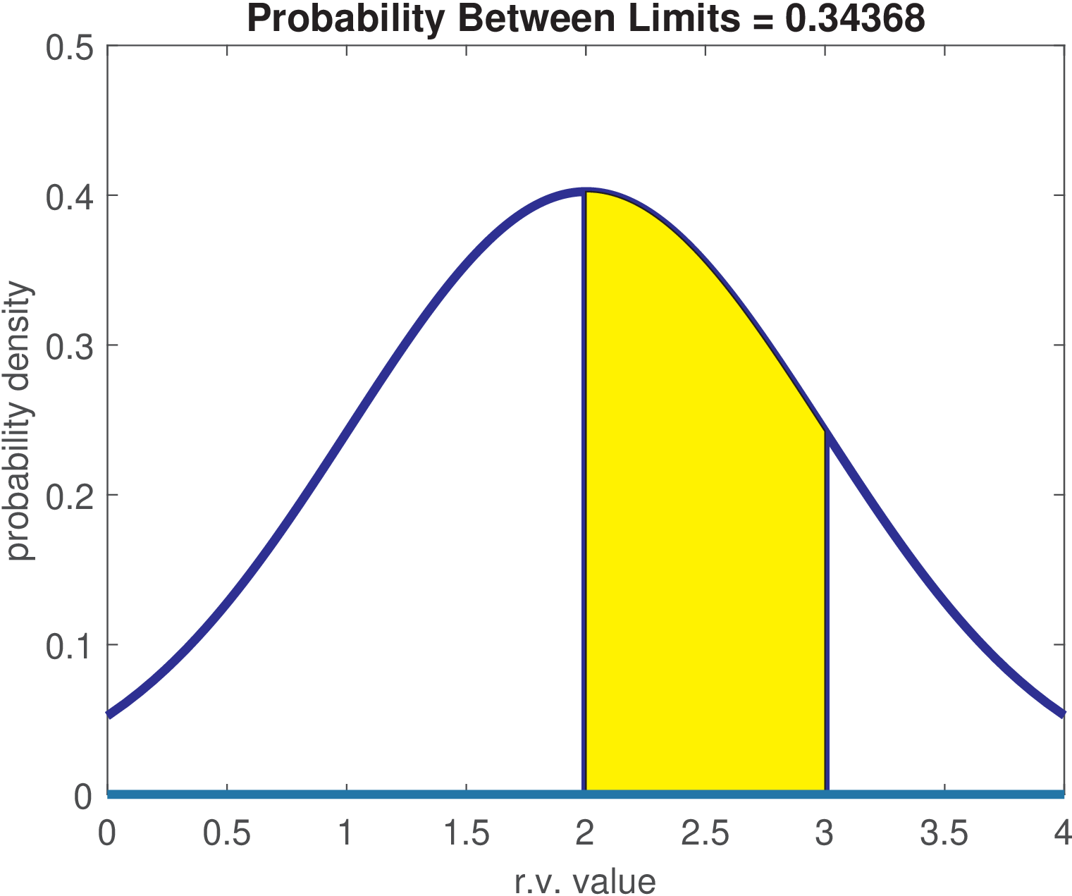
Now consider that $Y$ represents the amplitude of a Gaussian noise source with mean 2 and variance equal to 1. Its pdf is shown in Figure B.2. A common mistake is to assign a non-zero value to a specific value of a density function. For example, it is wrong to say that the probability of $Y=2$ is $0.4$, in spite of this being the value of the function. The function represents a density, and the correct answer is that the probability of $Y=2$, or any other point, is 0. One can extract probability from a pdf only integrating it over a non-zero range of its abscissa. For example, over the range [2, 3] the probability is approximately 0.34 as indicated by the shaded area in Figure B.2.

When dealing with ratios of pdfs it is possible to have the abscissa range ${\mathrm{\Delta }}_x$ canceling out. For example, if a discrete binary r.v. is used to represent two classes (A and B, for example), and each class has a pdf associated to it ($f(\mathbf{\text{x}}|A)$ and $f(\mathbf{\text{x}}|B)$, respectively), the Bayes’ rule states

In this case, ${\mathrm{\Delta }}_x$ cancels because it appears on both numerator and denominator.

B.3.3  Expected value

The expected value $𝔼[\cdot ]$ operator is the most common mathematical formalism for calculating an average (or mean).

The expected value is a linear operator (see Appendix B.7.1 for more information about linearity), such that

The expected value $𝔼[X]$ of a random variable $X$ can be estimated as a typical average when $X$ can be represented by a finite-dimension vector. For example, if $\mathbf{\text{x}}=[3,5,4,4,5,3]$ is a vector with random samples from $X$, the expected value $𝔼[X]$ can be estimated as $𝔼[X]\approx \overline{\mathbf{\text{x}}}=(3+5+4+4+5+3)∕6=4$, where $\overline{\mathbf{\text{x}}}$ is the conventional mean value.

If one has realizations of a random variable $X$, for instance organized as a vector $\mathbf{\text{x}}$, and is looking for the expected value $𝔼[g(X)]$ of a function $g(X)$, it is possible to apply the function $g(\cdot )$ to each realization (value of $\mathbf{\text{x}}$) and then take their average. For example, assume $g(X)=X^2$ and one is interested on estimating $𝔼[X^2]$ based on realizations $\mathbf{\text{x}}=[-1,3,-3,4,-2]$ of $X$. In this case, applying $g(X)=X^2$ to elements of $\mathbf{\text{x}}$ leads to the vector $\mathbf{\text{y}}=[{(-1)}^2,3^2,{(-3)}^2,4^2,{(-2)}^2]$, which has the average $\overline{\mathbf{\text{y}}}=(1+9+9+16+4)∕5=7.8$. The estimate is $𝔼[X^2]\approx \overline{\mathbf{\text{y}}}=7.8$.

As another example, consider ${\mu }_x=𝔼[X]$ is known (or has been previously estimated), and one is interested on estimating the variance $𝔼[{(X-{\mu }_x)}^2]$. In this case, $g(X)={(X-{\mu }_x)}^2$ and if the realizations are still $\mathbf{\text{x}}=[-1,3,-3,4,-2]$, which has an average ${\mu }_x=0.2$, applying $f(X)$ leads to a vector $\mathbf{\text{z}}=[{(-1-0.2)}^2,{(3-0.2)}^2,{(-3-0.2)}^2,{(4-0.2)}^2,{(-2-0.2)}^2]$ with mean value $\overline{\mathbf{\text{z}}}=7.76$. In this case the estimated variance is $𝔼[{(X-{\mu }_x)}^2]\approx \overline{\mathbf{\text{z}}}=7.76$.

The variance is often denoted as ${\sigma }_x^2$, and can be written as

which is often interpreted as $𝔼[X^2]={\sigma }_x^2+{\mu }_x^2$.

When a discrete random variable $X$ has $V$ distinct values, its mean $𝔼[X]$ can be estimated with

where $p_i$ is the probability of the $i$-th possible value $x_i$. For instance, the realizations $\mathbf{\text{x}}=[3,5,4,4,5,3]$ have only $V=3$ distinct values: $x_1=3,x_2=4$ and $x_3=5$, each one with estimated probability $p_i=1∕3,\forall <!--\; FUNCTION\; APPLICATION\; -->i$. Hence,

The same result could be obtained by directly taking the mean value of the $N=6$ elements with

Note that $x[n]$ corresponds to the $n$-th element in $\mathbf{\text{x}}$, while $x_i$ is the $i$-th distinct value of $\mathbf{\text{x}}$.

When $X\in ℝ$ is a continuous random variable, instead of Eq. (B.29) one has its continuous version:

where $f_X(x)$ is the probability density function of $X$. In this case, for each value of $x$, the role of the probability $p_i$ in the discrete r.v. case, is played by the value $f_X(x)$ that corresponds to a “weight” that depends on the likelihood of the specific value $x$.

In order to find $𝔼[g(X)]$ for a given function $g(\cdot )$ one can use:

B.3.4  Orthogonal versus uncorrelated

Two random variables $X$ and $Y$ are said to be orthogonal to each other if

They are said to be uncorrelated with each other if

The above condition is equivalent to

Note that if one or both of $X$ and $Y$ have zero mean, then the orthogonal and uncorrelated conditions are equivalent.

B.3.5  PDF of a sum of two independent random variables

If $X$ and $Y$ are independent random variables and $Z=X+Y$, then the probability density function (pdf) of $Z$ is given by the convolution

Example B.2. Probability distribution of noisy bipolar signal. As an example, consider a bipolar signal that takes values $\pm 5$ V with equal probability, whose pdf is

and additive white Gaussian noise (AWGN) with pdf $f_y(y)$. In this case, the pdf of $Z=X+Y$ is obtained by convolution and results in two shifted replicas of $f_y(y)$:

That is, the output pdf consists of two Gaussian components, each scaled by $1∕2$ and centered at $-5$ and $5$, respectively.   $\text{□}$